1 TL;DR
The 4th post in the Scientist’s Guide to R series introduces data transformation techniques useful for wrangling/tidying/cleaning data. Specifically, we will be learning how to use the 6 core functions (and a few others) from the popular dplyr package, perform similar operations in base R, and chain operations with the pipe operator (%>%) to streamline the process.
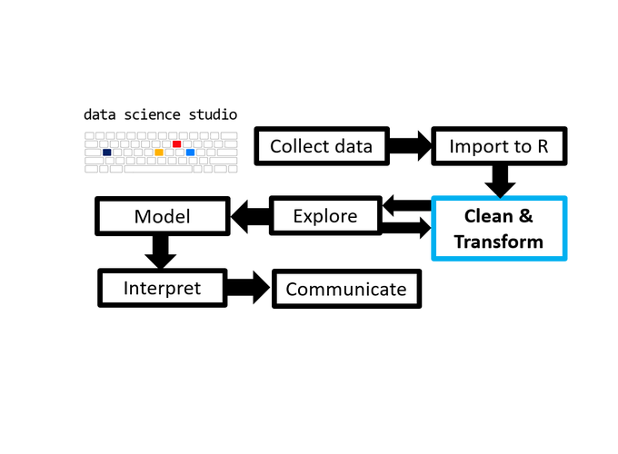
2 Introduction
The 4th post in the Scientist’s Guide to R series introduces data transformation techniques useful for wrangling/tidying/cleaning data, which often takes longer than any other step in the data analysis process. Specifically, we will be learning how to use the 6 core functions or “verbs” of the popular dplyr package to:
Easily select a subset of columns.
filter rows using logical tests with values of specified columns.
Modify columns or add new ones using mutate.
Obtain descriptive summaries of data using summarise (or the equivalent summarize()).
Assign a grouping structure to a data frame to enable subsequent dplyr package function calls to be executed within groups using group_by.
arrange a data frame for improved readability.
Some additional relevant functions that build on this foundation will also be covered where appropriate.
While other great packages (and other functions in base R) exist to help you manipulate data, using the dplyr package is perhaps the easiest way to learn these essential data processing techniques. However, if you find yourself working with very large datasets (e.g. > 1,000,000 rows) you might want to check out the data.table package, which emphasizes efficiency and performance over readability and ease of use.
Most dplyr functions accept a data frame or tibble as their first argument and return a data frame as their output. This is a key design feature that enables you to apply a series of operations to a data frame in a chain using the pipe operator (%>%), as demonstrated in section 8.
3 select()
select() is one of the dplyr functions you can use for subsetting. select() lets you extract a subset of columns from a data frame.
Columns may be specified using indices, names, or using string patterns with the assistance of a few tidyselect helper functions such as contains(), starts_with(), and ends_with().
library(dplyr) #load the dplyr package with the library function.##
## Attaching package: 'dplyr'## The following objects are masked from 'package:stats':
##
## filter, lag## The following objects are masked from 'package:base':
##
## intersect, setdiff, setequal, union#the dplyr package will be used throughout this tutorial so make sure it is
#loaded before trying to run the examples yourself
df <- starwars #assign the star wars data frame (imported when dplyr is loaded) to the label/name "df"
# inspect the structure
glimpse(df)## Rows: 87
## Columns: 14
## $ name <chr> "Luke Skywalker", "C-3PO", "R2-D2", "Darth Vader", "Leia Or~
## $ height <int> 172, 167, 96, 202, 150, 178, 165, 97, 183, 182, 188, 180, 2~
## $ mass <dbl> 77.0, 75.0, 32.0, 136.0, 49.0, 120.0, 75.0, 32.0, 84.0, 77.~
## $ hair_color <chr> "blond", NA, NA, "none", "brown", "brown, grey", "brown", N~
## $ skin_color <chr> "fair", "gold", "white, blue", "white", "light", "light", "~
## $ eye_color <chr> "blue", "yellow", "red", "yellow", "brown", "blue", "blue",~
## $ birth_year <dbl> 19.0, 112.0, 33.0, 41.9, 19.0, 52.0, 47.0, NA, 24.0, 57.0, ~
## $ sex <chr> "male", "none", "none", "male", "female", "male", "female",~
## $ gender <chr> "masculine", "masculine", "masculine", "masculine", "femini~
## $ homeworld <chr> "Tatooine", "Tatooine", "Naboo", "Tatooine", "Alderaan", "T~
## $ species <chr> "Human", "Droid", "Droid", "Human", "Human", "Human", "Huma~
## $ films <list> <"The Empire Strikes Back", "Revenge of the Sith", "Return~
## $ vehicles <list> <"Snowspeeder", "Imperial Speeder Bike">, <>, <>, <>, "Imp~
## $ starships <list> <"X-wing", "Imperial shuttle">, <>, <>, "TIE Advanced x1",~#in base R, you would extract columns using either [, "name"] or [["name"]], or $name
df[, "name"] #[] returns another data frame## # A tibble: 87 x 1
## name
## <chr>
## 1 Luke Skywalker
## 2 C-3PO
## 3 R2-D2
## 4 Darth Vader
## 5 Leia Organa
## 6 Owen Lars
## 7 Beru Whitesun lars
## 8 R5-D4
## 9 Biggs Darklighter
## 10 Obi-Wan Kenobi
## # ... with 77 more rowshead(df[["name"]]) #[[]] returns a 1 dimensional vector. head() just shows the 1st 6 values## [1] "Luke Skywalker" "C-3PO" "R2-D2" "Darth Vader"
## [5] "Leia Organa" "Owen Lars"df[, c("name", "mass", "hair_color")] #[] can accept a vector of names## # A tibble: 87 x 3
## name mass hair_color
## <chr> <dbl> <chr>
## 1 Luke Skywalker 77 blond
## 2 C-3PO 75 <NA>
## 3 R2-D2 32 <NA>
## 4 Darth Vader 136 none
## 5 Leia Organa 49 brown
## 6 Owen Lars 120 brown, grey
## 7 Beru Whitesun lars 75 brown
## 8 R5-D4 32 <NA>
## 9 Biggs Darklighter 84 black
## 10 Obi-Wan Kenobi 77 auburn, white
## # ... with 77 more rows#df[[c("name", "mass", "hair_color")]] #[[]] can't and returns an error
#or a logical or integer vector the same length as the number of columns
df[, 1:ncol(df) %% 2 == 0] #columns with even indices## # A tibble: 87 x 7
## height hair_color eye_color sex homeworld films starships
## <int> <chr> <chr> <chr> <chr> <list> <list>
## 1 172 blond blue male Tatooine <chr [5]> <chr [2]>
## 2 167 <NA> yellow none Tatooine <chr [6]> <chr [0]>
## 3 96 <NA> red none Naboo <chr [7]> <chr [0]>
## 4 202 none yellow male Tatooine <chr [4]> <chr [1]>
## 5 150 brown brown female Alderaan <chr [5]> <chr [0]>
## 6 178 brown, grey blue male Tatooine <chr [3]> <chr [0]>
## 7 165 brown blue female Tatooine <chr [3]> <chr [0]>
## 8 97 <NA> red none Tatooine <chr [1]> <chr [0]>
## 9 183 black brown male Tatooine <chr [1]> <chr [1]>
## 10 182 auburn, white blue-gray male Stewjon <chr [6]> <chr [5]>
## # ... with 77 more rowsdf[, 1:5] #1st 5 columns## # A tibble: 87 x 5
## name height mass hair_color skin_color
## <chr> <int> <dbl> <chr> <chr>
## 1 Luke Skywalker 172 77 blond fair
## 2 C-3PO 167 75 <NA> gold
## 3 R2-D2 96 32 <NA> white, blue
## 4 Darth Vader 202 136 none white
## 5 Leia Organa 150 49 brown light
## 6 Owen Lars 178 120 brown, grey light
## 7 Beru Whitesun lars 165 75 brown light
## 8 R5-D4 97 32 <NA> white, red
## 9 Biggs Darklighter 183 84 black light
## 10 Obi-Wan Kenobi 182 77 auburn, white fair
## # ... with 77 more rows#dplyr::select() makes extracting multiple columns even easier
select(df,
name, mass, hair_color) #note that names don't have to be quoted## # A tibble: 87 x 3
## name mass hair_color
## <chr> <dbl> <chr>
## 1 Luke Skywalker 77 blond
## 2 C-3PO 75 <NA>
## 3 R2-D2 32 <NA>
## 4 Darth Vader 136 none
## 5 Leia Organa 49 brown
## 6 Owen Lars 120 brown, grey
## 7 Beru Whitesun lars 75 brown
## 8 R5-D4 32 <NA>
## 9 Biggs Darklighter 84 black
## 10 Obi-Wan Kenobi 77 auburn, white
## # ... with 77 more rowsselect(df, name:hair_color) #and you can get all columns in a range using unquoted names## # A tibble: 87 x 4
## name height mass hair_color
## <chr> <int> <dbl> <chr>
## 1 Luke Skywalker 172 77 blond
## 2 C-3PO 167 75 <NA>
## 3 R2-D2 96 32 <NA>
## 4 Darth Vader 202 136 none
## 5 Leia Organa 150 49 brown
## 6 Owen Lars 178 120 brown, grey
## 7 Beru Whitesun lars 165 75 brown
## 8 R5-D4 97 32 <NA>
## 9 Biggs Darklighter 183 84 black
## 10 Obi-Wan Kenobi 182 77 auburn, white
## # ... with 77 more rowsselect(df, 1:5, 9, 10) #select also accepts column indices and doesn't require c()## # A tibble: 87 x 7
## name height mass hair_color skin_color gender homeworld
## <chr> <int> <dbl> <chr> <chr> <chr> <chr>
## 1 Luke Skywalker 172 77 blond fair masculine Tatooine
## 2 C-3PO 167 75 <NA> gold masculine Tatooine
## 3 R2-D2 96 32 <NA> white, blue masculine Naboo
## 4 Darth Vader 202 136 none white masculine Tatooine
## 5 Leia Organa 150 49 brown light feminine Alderaan
## 6 Owen Lars 178 120 brown, grey light masculine Tatooine
## 7 Beru Whitesun lars 165 75 brown light feminine Tatooine
## 8 R5-D4 97 32 <NA> white, red masculine Tatooine
## 9 Biggs Darklighter 183 84 black light masculine Tatooine
## 10 Obi-Wan Kenobi 182 77 auburn, white fair masculine Stewjon
## # ... with 77 more rows#select everything other than a specified column using the subtraction operator "-"
select(df, -hair_color, -mass) ## # A tibble: 87 x 12
## name height skin_color eye_color birth_year sex gender homeworld species
## <chr> <int> <chr> <chr> <dbl> <chr> <chr> <chr> <chr>
## 1 Luke S~ 172 fair blue 19 male mascu~ Tatooine Human
## 2 C-3PO 167 gold yellow 112 none mascu~ Tatooine Droid
## 3 R2-D2 96 white, bl~ red 33 none mascu~ Naboo Droid
## 4 Darth ~ 202 white yellow 41.9 male mascu~ Tatooine Human
## 5 Leia O~ 150 light brown 19 fema~ femin~ Alderaan Human
## 6 Owen L~ 178 light blue 52 male mascu~ Tatooine Human
## 7 Beru W~ 165 light blue 47 fema~ femin~ Tatooine Human
## 8 R5-D4 97 white, red red NA none mascu~ Tatooine Droid
## 9 Biggs ~ 183 light brown 24 male mascu~ Tatooine Human
## 10 Obi-Wa~ 182 fair blue-gray 57 male mascu~ Stewjon Human
## # ... with 77 more rows, and 3 more variables: films <list>, vehicles <list>,
## # starships <list>select(df, -c(name:hair_color)) #everything other than a range of named columns## # A tibble: 87 x 10
## skin_color eye_color birth_year sex gender homeworld species films vehicles
## <chr> <chr> <dbl> <chr> <chr> <chr> <chr> <lis> <list>
## 1 fair blue 19 male mascu~ Tatooine Human <chr~ <chr [2~
## 2 gold yellow 112 none mascu~ Tatooine Droid <chr~ <chr [0~
## 3 white, bl~ red 33 none mascu~ Naboo Droid <chr~ <chr [0~
## 4 white yellow 41.9 male mascu~ Tatooine Human <chr~ <chr [0~
## 5 light brown 19 fema~ femin~ Alderaan Human <chr~ <chr [1~
## 6 light blue 52 male mascu~ Tatooine Human <chr~ <chr [0~
## 7 light blue 47 fema~ femin~ Tatooine Human <chr~ <chr [0~
## 8 white, red red NA none mascu~ Tatooine Droid <chr~ <chr [0~
## 9 light brown 24 male mascu~ Tatooine Human <chr~ <chr [0~
## 10 fair blue-gray 57 male mascu~ Stewjon Human <chr~ <chr [1~
## # ... with 77 more rows, and 1 more variable: starships <list># dplyr also provides a number of "select helper" functions that allow you to
# select variables using string patterns, e.g.
select(df, contains("m")) #all columns with names that contain the letter m## # A tibble: 87 x 4
## name mass homeworld films
## <chr> <dbl> <chr> <list>
## 1 Luke Skywalker 77 Tatooine <chr [5]>
## 2 C-3PO 75 Tatooine <chr [6]>
## 3 R2-D2 32 Naboo <chr [7]>
## 4 Darth Vader 136 Tatooine <chr [4]>
## 5 Leia Organa 49 Alderaan <chr [5]>
## 6 Owen Lars 120 Tatooine <chr [3]>
## 7 Beru Whitesun lars 75 Tatooine <chr [3]>
## 8 R5-D4 32 Tatooine <chr [1]>
## 9 Biggs Darklighter 84 Tatooine <chr [1]>
## 10 Obi-Wan Kenobi 77 Stewjon <chr [6]>
## # ... with 77 more rowsselect(df, starts_with("m")) #all columns with names that start with the letter m ## # A tibble: 87 x 1
## mass
## <dbl>
## 1 77
## 2 75
## 3 32
## 4 136
## 5 49
## 6 120
## 7 75
## 8 32
## 9 84
## 10 77
## # ... with 77 more rowsselect(df, ends_with("s")) #all columns with names that end with the letter s ## # A tibble: 87 x 5
## mass species films vehicles starships
## <dbl> <chr> <list> <list> <list>
## 1 77 Human <chr [5]> <chr [2]> <chr [2]>
## 2 75 Droid <chr [6]> <chr [0]> <chr [0]>
## 3 32 Droid <chr [7]> <chr [0]> <chr [0]>
## 4 136 Human <chr [4]> <chr [0]> <chr [1]>
## 5 49 Human <chr [5]> <chr [1]> <chr [0]>
## 6 120 Human <chr [3]> <chr [0]> <chr [0]>
## 7 75 Human <chr [3]> <chr [0]> <chr [0]>
## 8 32 Droid <chr [1]> <chr [0]> <chr [0]>
## 9 84 Human <chr [1]> <chr [0]> <chr [1]>
## 10 77 Human <chr [6]> <chr [1]> <chr [5]>
## # ... with 77 more rows# there is also a select helper called "matches" that enables you to select columns
# with more complex string patterns using regular expressions
# a detailed introduction to the "matches" select helper, string manipulation,
# and regular expressions will be covered in a later post.
# see the documentation for select_helpers (from the tidyselect package, which
# is loaded with dplyr) for more info
# ?tidyselect::select_helpers
# you can rearrange columns and rename them during the selection process
select(df, 5:last_col(), 1:4) #select columns 5 to the end, then columns 1 to 4 ## # A tibble: 87 x 14
## skin_color eye_color birth_year sex gender homeworld species films vehicles
## <chr> <chr> <dbl> <chr> <chr> <chr> <chr> <lis> <list>
## 1 fair blue 19 male mascu~ Tatooine Human <chr~ <chr [2~
## 2 gold yellow 112 none mascu~ Tatooine Droid <chr~ <chr [0~
## 3 white, bl~ red 33 none mascu~ Naboo Droid <chr~ <chr [0~
## 4 white yellow 41.9 male mascu~ Tatooine Human <chr~ <chr [0~
## 5 light brown 19 fema~ femin~ Alderaan Human <chr~ <chr [1~
## 6 light blue 52 male mascu~ Tatooine Human <chr~ <chr [0~
## 7 light blue 47 fema~ femin~ Tatooine Human <chr~ <chr [0~
## 8 white, red red NA none mascu~ Tatooine Droid <chr~ <chr [0~
## 9 light brown 24 male mascu~ Tatooine Human <chr~ <chr [0~
## 10 fair blue-gray 57 male mascu~ Stewjon Human <chr~ <chr [1~
## # ... with 77 more rows, and 5 more variables: starships <list>, name <chr>,
## # height <int>, mass <dbl>, hair_color <chr># to select() a single column and turn it into a vector (instead of leaving it as a data frame),
all.equal(
pull(select(df, mass), mass), # wrap it in the pull function (also from dplyr)
df$mass, # or use the $ symbol
df[["mass"]] # or the equivalent `[[` operator
)## [1] TRUE3.1 Renaming Columns with select() or rename()
Columns can also be renamed when subsetting with the select() function or without subsetting using the rename() function (also in the dplyr package).
#rename and subset using select
select(df, nm = name, hgt = height, byear = birth_year) #select columns and rename them## # A tibble: 87 x 3
## nm hgt byear
## <chr> <int> <dbl>
## 1 Luke Skywalker 172 19
## 2 C-3PO 167 112
## 3 R2-D2 96 33
## 4 Darth Vader 202 41.9
## 5 Leia Organa 150 19
## 6 Owen Lars 178 52
## 7 Beru Whitesun lars 165 47
## 8 R5-D4 97 NA
## 9 Biggs Darklighter 183 24
## 10 Obi-Wan Kenobi 182 57
## # ... with 77 more rows#to just rename columns without subsetting, use dplyr::rename() instead of select()
rename(df, nm = name, hgt = height, b_year = birth_year) #returns all columns## # A tibble: 87 x 14
## nm hgt mass hair_color skin_color eye_color b_year sex gender
## <chr> <int> <dbl> <chr> <chr> <chr> <dbl> <chr> <chr>
## 1 Luke Skyw~ 172 77 blond fair blue 19 male mascul~
## 2 C-3PO 167 75 <NA> gold yellow 112 none mascul~
## 3 R2-D2 96 32 <NA> white, bl~ red 33 none mascul~
## 4 Darth Vad~ 202 136 none white yellow 41.9 male mascul~
## 5 Leia Orga~ 150 49 brown light brown 19 fema~ femini~
## 6 Owen Lars 178 120 brown, grey light blue 52 male mascul~
## 7 Beru Whit~ 165 75 brown light blue 47 fema~ femini~
## 8 R5-D4 97 32 <NA> white, red red NA none mascul~
## 9 Biggs Dar~ 183 84 black light brown 24 male mascul~
## 10 Obi-Wan K~ 182 77 auburn, whi~ fair blue-gray 57 male mascul~
## # ... with 77 more rows, and 5 more variables: homeworld <chr>, species <chr>,
## # films <list>, vehicles <list>, starships <list>#to save the updated names just assign the output back to the same data frame object
renamed_df <- rename(df, nm = name, hgt = height, b_year = birth_year)
#In base R you can just assign names using a string vector.
#The main disadvantage of this method is that all variable names have to be specified,
#instead of just the ones that you want to change (which is all you need to do with the rename function)
#Unlike select() or rename(), the base R method also requires that names be assigned in the correct order,
#according to the column indices.
df_names <- names(df) #store the original names
names(df) <- c("nm", "hgt", "mass",
"hair_color", "skin_color", "eye_color",
"b_year") #returns a warning and then all non-specified names become NA## Warning: The `value` argument of `names<-` must have the same length as `x` as of tibble 3.0.0.
## `names` must have length 14, not 7.## Warning: The `value` argument of `names<-` can't be empty as of tibble 3.0.0.
## Columns 8, 9, 10, 11, 12, and 2 more must be named.names(df) <- df_names #restore the original names from the vector saved above4 filter()
filter() is the other core dplyr verb you can use for subsetting your data. filter() lets you extract a subset of rows using logical operators.
To filter a data frame, specify the name of the data frame as the 1st argument, then any number of logical tests for values of variables in the data frame that you want to use as filtering criteria.
# we'll just work with a few columns to simplify the output and highlight the filtering
df2 <- select(df, name, height, species, homeworld)

unique(df2$homeworld) #check the unique values of the homeworld variable, which we will use for filtering
## [1] "Tatooine" "Naboo" "Alderaan" "Stewjon"
## [5] "Eriadu" "Kashyyyk" "Corellia" "Rodia"
## [9] "Nal Hutta" "Bestine IV" NA "Kamino"
## [13] "Trandosha" "Socorro" "Bespin" "Mon Cala"
## [17] "Chandrila" "Endor" "Sullust" "Cato Neimoidia"
## [21] "Coruscant" "Toydaria" "Malastare" "Dathomir"
## [25] "Ryloth" "Vulpter" "Troiken" "Tund"
## [29] "Haruun Kal" "Cerea" "Glee Anselm" "Iridonia"
## [33] "Iktotch" "Quermia" "Dorin" "Champala"
## [37] "Geonosis" "Mirial" "Serenno" "Concord Dawn"
## [41] "Zolan" "Ojom" "Aleen Minor" "Skako"
## [45] "Muunilinst" "Shili" "Kalee" "Umbara"
## [49] "Utapau"# use filter to get a subset of all star wars characters from either Tatooine or Naboo
filter(df2,
homeworld == "Tatooine" | homeworld == "Naboo") #recall that the vertical bar `|` is the logical operator 'or'## # A tibble: 21 x 4
## name height species homeworld
## <chr> <int> <chr> <chr>
## 1 Luke Skywalker 172 Human Tatooine
## 2 C-3PO 167 Droid Tatooine
## 3 R2-D2 96 Droid Naboo
## 4 Darth Vader 202 Human Tatooine
## 5 Owen Lars 178 Human Tatooine
## 6 Beru Whitesun lars 165 Human Tatooine
## 7 R5-D4 97 Droid Tatooine
## 8 Biggs Darklighter 183 Human Tatooine
## 9 Anakin Skywalker 188 Human Tatooine
## 10 Palpatine 170 Human Naboo
## # ... with 11 more rows# this is read: filter the data frame "df2" to extract rows where the value of
# the variable homeworld is equal to "Tatooine" or homeworld is equal to "Naboo"
#in base R, one equivalent option would be:
df2[(df2$homeworld == "Tatooine" | df2$homeworld == "Naboo"), ]## # A tibble: 31 x 4
## name height species homeworld
## <chr> <int> <chr> <chr>
## 1 Luke Skywalker 172 Human Tatooine
## 2 C-3PO 167 Droid Tatooine
## 3 R2-D2 96 Droid Naboo
## 4 Darth Vader 202 Human Tatooine
## 5 Owen Lars 178 Human Tatooine
## 6 Beru Whitesun lars 165 Human Tatooine
## 7 R5-D4 97 Droid Tatooine
## 8 Biggs Darklighter 183 Human Tatooine
## 9 Anakin Skywalker 188 Human Tatooine
## 10 <NA> NA <NA> <NA>
## # ... with 21 more rows# notice that the $ is not needed to specify which data set the variable
# "homeworld" is in for filter but it is if you are passing a logical vector to
# subset a data frame using `[]` in base R
# this is because R reads (df2$homeworld == "Tatooine" | df2$homeworld == "Naboo")
# as a logical test and returns a logical vector, which is then used to specify
# which rows to extract (those with values == TRUE) and which to discard (those
# with values == FALSE). This becomes really clear if you just pull out the
# subsetting predicates and print the result
(df2$homeworld == "Tatooine" | df2$homeworld == "Naboo")## [1] TRUE TRUE TRUE TRUE FALSE TRUE TRUE TRUE TRUE FALSE TRUE FALSE
## [13] FALSE FALSE FALSE FALSE FALSE FALSE NA TRUE FALSE NA FALSE FALSE
## [25] FALSE FALSE FALSE NA FALSE FALSE NA FALSE FALSE TRUE TRUE TRUE
## [37] TRUE FALSE FALSE TRUE TRUE FALSE FALSE FALSE FALSE FALSE FALSE FALSE
## [49] FALSE FALSE FALSE FALSE FALSE FALSE FALSE FALSE TRUE TRUE TRUE FALSE
## [61] FALSE FALSE TRUE FALSE FALSE FALSE FALSE FALSE FALSE FALSE FALSE FALSE
## [73] NA FALSE FALSE FALSE FALSE FALSE FALSE FALSE FALSE NA NA NA
## [85] NA NA TRUE# to get indices instead of logical values, you can wrap the above in which(), e.g.
ind <- which(df2$homeworld == "Tatooine" | df2$homeworld == "Naboo") #returns the indices where the criteria are TRUE
ind #calling an object itself without applying any functions to it just prints it to the console## [1] 1 2 3 4 6 7 8 9 11 20 34 35 36 37 40 41 57 58 59 63 87#note that you could also pass a vector of integers to subset a df2 using `[]`
df2[ind, ]## # A tibble: 21 x 4
## name height species homeworld
## <chr> <int> <chr> <chr>
## 1 Luke Skywalker 172 Human Tatooine
## 2 C-3PO 167 Droid Tatooine
## 3 R2-D2 96 Droid Naboo
## 4 Darth Vader 202 Human Tatooine
## 5 Owen Lars 178 Human Tatooine
## 6 Beru Whitesun lars 165 Human Tatooine
## 7 R5-D4 97 Droid Tatooine
## 8 Biggs Darklighter 183 Human Tatooine
## 9 Anakin Skywalker 188 Human Tatooine
## 10 Palpatine 170 Human Naboo
## # ... with 11 more rows#to negate a logical test, you can use `!` which means "not"
# in the context of subsetting, this negates a logical vector
!(df2$homeworld == "Tatooine" | df2$homeworld == "Naboo")## [1] FALSE FALSE FALSE FALSE TRUE FALSE FALSE FALSE FALSE TRUE FALSE TRUE
## [13] TRUE TRUE TRUE TRUE TRUE TRUE NA FALSE TRUE NA TRUE TRUE
## [25] TRUE TRUE TRUE NA TRUE TRUE NA TRUE TRUE FALSE FALSE FALSE
## [37] FALSE TRUE TRUE FALSE FALSE TRUE TRUE TRUE TRUE TRUE TRUE TRUE
## [49] TRUE TRUE TRUE TRUE TRUE TRUE TRUE TRUE FALSE FALSE FALSE TRUE
## [61] TRUE TRUE FALSE TRUE TRUE TRUE TRUE TRUE TRUE TRUE TRUE TRUE
## [73] NA TRUE TRUE TRUE TRUE TRUE TRUE TRUE TRUE NA NA NA
## [85] NA NA FALSE#this is why the logical test for not equal to is "!="
identical(!(df2$homeworld == "Tatooine"), df2$homeworld != "Tatooine") #use identical() or all.equal() to test for equality between entire R objects## [1] TRUE# extract rows for characters who are at least 100 cm tall and are from Naboo
filter(df2, height >= 100 & homeworld == "Naboo")## # A tibble: 10 x 4
## name height species homeworld
## <chr> <int> <chr> <chr>
## 1 Palpatine 170 Human Naboo
## 2 Jar Jar Binks 196 Gungan Naboo
## 3 Roos Tarpals 224 Gungan Naboo
## 4 Rugor Nass 206 Gungan Naboo
## 5 Ric Olié 183 <NA> Naboo
## 6 Quarsh Panaka 183 <NA> Naboo
## 7 Gregar Typho 185 Human Naboo
## 8 Cordé 157 Human Naboo
## 9 Dormé 165 Human Naboo
## 10 Padmé Amidala 165 Human Naboo# when using filter(), you can substitute a comma for `&` when specifying multiple criteria
identical(filter(df2, height >= 100 & homeworld == "Naboo"),
filter(df2, height >= 100, homeworld == "Naboo"))## [1] TRUE# multiple or (`|`) clauses can instead be specified using the %in% infix operator
option1 <- filter(df2, homeworld == "Tatooine" | homeworld == "Naboo" | homeworld == "Alderaan")
option2 <- filter(filter(df2, homeworld %in% c("Tatooine", "Naboo", "Alderaan")))
identical(option1, option2)## [1] TRUE# since %in% also returns a logical vector, it can also be negated using `!`,
# although they give different results if the data contain missing values (NA)
a <- !(df2$homeworld == "Tatooine" | df2$homeworld == "Naboo" | df2$homeworld == "Alderaan")
b <- !(df2$homeworld %in% c("Tatooine", "Naboo", "Alderaan"))
all.equal(a, b)## [1] "'is.NA' value mismatch: 0 in current 10 in target"b[is.na(a)] #these missing values were converted to TRUE by %in%## [1] TRUE TRUE TRUE TRUE TRUE TRUE TRUE TRUE TRUE TRUE# to avoid this and other problems many functions have with processing NA
# values, it is often best to either remove them or impute them, or use the
# na.rm argument for the function
x <- na.omit(df2$homeworld)
c <- !(x == "Tatooine" | x == "Naboo" | x == "Alderaan")
# negating a set of `or` clauses for equality is the same as multiple `and`
# clauses for inequality
d <- x != "Tatooine" & x != "Naboo" & x != "Alderaan"
e <- !(x %in% c("Tatooine", "Naboo", "Alderaan"))
all.equal(c, d, e)## [1] TRUE# key point: you can use logical comparisons and vectors for subsetting in R4.1 Subset Rows using Indices with slice()
Unlike select(), filter() doesn’t allow the use of indices for subsetting. Instead, dplyr has another funciton called slice() for this purpose. slice() doesn’t require you to enclose multiple index values in c() either and it can also operate on indices within groups (see the section 7 below for an example).
slice(df2, 1:5, 9:14, 25:50)## # A tibble: 37 x 4
## name height species homeworld
## <chr> <int> <chr> <chr>
## 1 Luke Skywalker 172 Human Tatooine
## 2 C-3PO 167 Droid Tatooine
## 3 R2-D2 96 Droid Naboo
## 4 Darth Vader 202 Human Tatooine
## 5 Leia Organa 150 Human Alderaan
## 6 Biggs Darklighter 183 Human Tatooine
## 7 Obi-Wan Kenobi 182 Human Stewjon
## 8 Anakin Skywalker 188 Human Tatooine
## 9 Wilhuff Tarkin 180 Human Eriadu
## 10 Chewbacca 228 Wookiee Kashyyyk
## # ... with 27 more rows5 mutate()
mutate() lets you modify and/or create new columns in a data frame.
#Say for example that you wanted to calculate the BMI of each character in the starwars data frame

df2 <- select(df, name, height, mass) #extract columns of interest

df3 <- mutate(df2,
       height_in_m  = height/100, #convert height from cm to m, store in new column "height_in_m"
       bmi = mass/(height_in_m^2), #add a column called bmi for the calculated body mass index of each character
       bmi = signif(bmi, 1)) #round it to one significant digit/decimal place & assign back to the same name.
df3## # A tibble: 87 x 5
## name height mass height_in_m bmi
## <chr> <int> <dbl> <dbl> <dbl>
## 1 Luke Skywalker 172 77 1.72 30
## 2 C-3PO 167 75 1.67 30
## 3 R2-D2 96 32 0.96 30
## 4 Darth Vader 202 136 2.02 30
## 5 Leia Organa 150 49 1.5 20
## 6 Owen Lars 178 120 1.78 40
## 7 Beru Whitesun lars 165 75 1.65 30
## 8 R5-D4 97 32 0.97 30
## 9 Biggs Darklighter 183 84 1.83 30
## 10 Obi-Wan Kenobi 182 77 1.82 20
## # ... with 77 more rows# assigning a modified variable to the same name overwrites/modifies the column
# note in the above mutate statement I created a new variable then used it in the same function call.
# this is possible because mutate() evaluates items from left to right
# the equivalent operations in base R would typically involve several steps
# requiring separate assignment of intermediate objects
df2$height_in_m <- df2$height/100
df2$bmi <- df2$mass/(df2$height_in_m^2)
df2$bmi <- signif(df2$bmi, 1)
all.equal(df2, df3)## [1] TRUE# As shown above, mutate lets you combine these steps into a single function call and doesn't
# require you to specify the dataframe$ component multiple times, you only have
# to supply the name of the data frame as the 1st argument.
# the transmute function (also in the dplyr package) is an alternative to mutate that
# only retains variables you specify (i.e. it combines select and mutate in a single step)
# You probably won't use it as often as mutate, but it can be helpful occassionally
transmute(df2,
height_in_m = height/100, #convert height from cm to m, store in new column "height_in_m"
bmi = mass/(height_in_m^2), #add a column called bmi for the calculated body mass index of each character
bmi = signif(bmi, 1))## # A tibble: 87 x 2
## height_in_m bmi
## <dbl> <dbl>
## 1 1.72 30
## 2 1.67 30
## 3 0.96 30
## 4 2.02 30
## 5 1.5 20
## 6 1.78 40
## 7 1.65 30
## 8 0.97 30
## 9 1.83 30
## 10 1.82 20
## # ... with 77 more rows5.1 Recoding or Creating Indicator Variables using if_else(), case_when(), or recode()
A common use of mutate (or transmute) is to encode a new variable (or overwrite an existing one) based on values of an existing variable in a data frame using the recode(), if_else() or case_when() functions in the dplyr package.
if_else() is a condensed version of a simple if/else statement with only 2 outcomes: one if the condition specified as the 1st argument evaluates to TRUE and one if it evaluates to FALSE (i.e. no else if components). case_when() lets you use multiple if_else() calls together without having to nest them explicitly. General control flow operations using conditional statments (if, else, else if, etc.) may be covered in a later blog post… For now I recommend this section of the advanced R book for those who want to learn more about it before moving on.
# to create an indicator/dummy/2-level variable (e.g. 1/0, T/F) you can use
# if_else() (or ifelse()):

if_else(df$height > 180, #part 1. logical test
        "tall", #part 2. value if TRUE
        "short") #part 3. value if FALSE (should be same class as the value if TRUE)
## [1] "short" "short" "short" "tall" "short" "short" "short" "short" "tall"
## [10] "tall" "tall" "short" "tall" "short" "short" "short" "short" "short"
## [19] "short" "short" "tall" "tall" "tall" "short" "short" "short" "short"
## [28] NA "short" "short" "tall" "tall" "short" "tall" "tall" "tall"
## [37] "tall" "short" "short" "tall" "short" "short" "short" "short" "short"
## [46] "short" "short" "tall" "tall" "tall" "short" "tall" "tall" "tall"
## [55] "tall" "tall" "tall" "short" "tall" "tall" "short" "short" "short"
## [64] "tall" "tall" "tall" "short" "tall" "tall" "tall" "short" "short"
## [73] "short" "tall" "tall" "short" "tall" "tall" "tall" "short" "tall"
## [82] NA NA NA NA NA "short"# use mutate to add it to an existing data frame
mutate(select(df, name, height), #apply mutate to a subset of the data using a nested select call
tall_or_short = if_else(height > 180,
"tall",
"short")) ## # A tibble: 87 x 3
## name height tall_or_short
## <chr> <int> <chr>
## 1 Luke Skywalker 172 short
## 2 C-3PO 167 short
## 3 R2-D2 96 short
## 4 Darth Vader 202 tall
## 5 Leia Organa 150 short
## 6 Owen Lars 178 short
## 7 Beru Whitesun lars 165 short
## 8 R5-D4 97 short
## 9 Biggs Darklighter 183 tall
## 10 Obi-Wan Kenobi 182 tall
## # ... with 77 more rows# to specify more than 2 conditions/outputs you can use case_when():
mutate(select(df, name, height),
size_class = case_when(height > 200 ~ "tall", #logical_test ~ value_if_TRUE,
height < 200 & height > 100 ~ "medium",
height < 100 ~ "short")
) ## # A tibble: 87 x 3
## name height size_class
## <chr> <int> <chr>
## 1 Luke Skywalker 172 medium
## 2 C-3PO 167 medium
## 3 R2-D2 96 short
## 4 Darth Vader 202 tall
## 5 Leia Organa 150 medium
## 6 Owen Lars 178 medium
## 7 Beru Whitesun lars 165 medium
## 8 R5-D4 97 short
## 9 Biggs Darklighter 183 medium
## 10 Obi-Wan Kenobi 182 medium
## # ... with 77 more rows# you can recode a variable using recode():
recoded_using_recode <- mutate(select(df, name, hair_color),
hair_color = recode(hair_color, #the variable you want to recode
"blond" = "BLOND",#old_value = new_value
"brown" = "BROWN") #you can recode any number of values this way
#unspecified values are unaltered
)
recoded_using_recode## # A tibble: 87 x 2
## name hair_color
## <chr> <chr>
## 1 Luke Skywalker BLOND
## 2 C-3PO <NA>
## 3 R2-D2 <NA>
## 4 Darth Vader none
## 5 Leia Organa BROWN
## 6 Owen Lars brown, grey
## 7 Beru Whitesun lars BROWN
## 8 R5-D4 <NA>
## 9 Biggs Darklighter black
## 10 Obi-Wan Kenobi auburn, white
## # ... with 77 more rows# unforunately, unlike other dplyr functions, recode()-ed values are specified as
# "old_value" = "new_value" instead of the more common "new" = "old" scheme used
# by select() and rename()
# an alternative would be to use case_when(), e.g.:
recoded_using_case_when <- mutate(select(df, name, hair_color),
hair_color = case_when(hair_color == "blond" ~ "BLOND",
hair_color == "brown" ~ "BROWN",
TRUE ~ as.character(hair_color)))
identical(recoded_using_recode, recoded_using_case_when) ## [1] TRUE# This time we add in the "TRUE ~ as.character(hair_color)" part to signify that
# all other non-NA cases should be the existing value of hair color as a
# character string; otherwise non-matching values are coded as missing values (`NA`)
# note that recode, like most R functions, returns a copy of the data object,
# that you have to assign to a name if you want to save it in the environment
#of course you can also recode variables in base R using the assingnment operator:
#`<-` (keyboard shortcut = )
df$hair_color[df$hair_color == "blond"] <- "BLOND"
df$hair_color[df$hair_color == "brown"] <- "BROWN"
#but this modifies the data frame in place, which isn't always what you want
#e.g. if you are just experimenting with a coding scheme and then decide you
#want to change it back you'll have to rerun earlier portions of your R script
#to recover the previous version6 summarise()
summarise() makes it easy to turn a data frame into a smaller data frame of summary statistics.
summary1 <- summarise(df, #as for the other dplyr functions, the data source is specified as the 1st argument
                      n = n(), #n() is a special function for use in summarize that returns the number of values
                      mean_height = mean(height, na.rm = TRUE), #summary stat name in the output = function(column) in the input
                      median_mass = median(mass, na.rm = TRUE))

summary1## # A tibble: 1 x 3
## n mean_height median_mass
## <int> <dbl> <dbl>
## 1 87 174. 79#summarise() and summarize() do the same thing and just accommodate different user spelling preferences
summary2 <- summarize(df, #as for the other dplyr functions, the data source is specified as the 1st argument
n = n(), #n() is a special function for use in summarize that returns the number of values
mean_height = mean(height, na.rm = TRUE), #summary stat name in the output = function(column) in the input
median_mass = median(mass, na.rm = TRUE))
identical(summary1, summary2)## [1] TRUE7 group_by()
group_by() adds an explicit grouping structure to a data frame that can subsequently be used by other dplyr functions to perform operations within each level of the grouping variable or level combination of the grouping variables if you specify multiple grouping variables. This is particularly useful in conjunction with either summarize() or mutate(), enabling you to calculate summary statistics or transform variables separately for each of the groups defined by group_by().
#structure of the data before grouping
glimpse(df)
## Rows: 87
## Columns: 14
## $ name <chr> "Luke Skywalker", "C-3PO", "R2-D2", "Darth Vader", "Leia Or~
## $ height <int> 172, 167, 96, 202, 150, 178, 165, 97, 183, 182, 188, 180, 2~
## $ mass <dbl> 77.0, 75.0, 32.0, 136.0, 49.0, 120.0, 75.0, 32.0, 84.0, 77.~
## $ hair_color <chr> "BLOND", NA, NA, "none", "BROWN", "brown, grey", "BROWN", N~
## $ skin_color <chr> "fair", "gold", "white, blue", "white", "light", "light", "~
## $ eye_color <chr> "blue", "yellow", "red", "yellow", "brown", "blue", "blue",~
## $ birth_year <dbl> 19.0, 112.0, 33.0, 41.9, 19.0, 52.0, 47.0, NA, 24.0, 57.0, ~
## $ sex <chr> "male", "none", "none", "male", "female", "male", "female",~
## $ gender <chr> "masculine", "masculine", "masculine", "masculine", "femini~
## $ homeworld <chr> "Tatooine", "Tatooine", "Naboo", "Tatooine", "Alderaan", "T~
## $ species <chr> "Human", "Droid", "Droid", "Human", "Human", "Human", "Huma~
## $ films <list> <"The Empire Strikes Back", "Revenge of the Sith", "Return~
## $ vehicles <list> <"Snowspeeder", "Imperial Speeder Bike">, <>, <>, <>, "Imp~
## $ starships <list> <"X-wing", "Imperial shuttle">, <>, <>, "TIE Advanced x1",~df3 <- select(df, name, species, height, mass)#1st. extract just the columns of interest
grouped_data <- group_by(df3, species) #group the data frame "df3" by the variable "species"
class(grouped_data) #new additional class = "grouped_df"## [1] "grouped_df" "tbl_df" "tbl" "data.frame"glimpse(grouped_data) #note that the structure now has a groups attribute## Rows: 87
## Columns: 4
## Groups: species [38]
## $ name <chr> "Luke Skywalker", "C-3PO", "R2-D2", "Darth Vader", "Leia Organ~
## $ species <chr> "Human", "Droid", "Droid", "Human", "Human", "Human", "Human",~
## $ height <int> 172, 167, 96, 202, 150, 178, 165, 97, 183, 182, 188, 180, 228,~
## $ mass <dbl> 77.0, 75.0, 32.0, 136.0, 49.0, 120.0, 75.0, 32.0, 84.0, 77.0, ~slice(grouped_data, 1) #look at the 1st row of each group## # A tibble: 38 x 4
## # Groups: species [38]
## name species height mass
## <chr> <chr> <int> <dbl>
## 1 Ratts Tyerell Aleena 79 15
## 2 Dexter Jettster Besalisk 198 102
## 3 Ki-Adi-Mundi Cerean 198 82
## 4 Mas Amedda Chagrian 196 NA
## 5 Zam Wesell Clawdite 168 55
## 6 C-3PO Droid 167 75
## 7 Sebulba Dug 112 40
## 8 Wicket Systri Warrick Ewok 88 20
## 9 Poggle the Lesser Geonosian 183 80
## 10 Jar Jar Binks Gungan 196 66
## # ... with 28 more rows#next summarise calculates the specified summary statistics within species
summarise(grouped_data,
n = n(),
mean_height = mean(height, na.rm = TRUE),
median_mass = median(mass, na.rm = TRUE))## `summarise()` ungrouping output (override with `.groups` argument)## # A tibble: 38 x 4
## species n mean_height median_mass
## <chr> <int> <dbl> <dbl>
## 1 Aleena 1 79 15
## 2 Besalisk 1 198 102
## 3 Cerean 1 198 82
## 4 Chagrian 1 196 NA
## 5 Clawdite 1 168 55
## 6 Droid 6 131. 53.5
## 7 Dug 1 112 40
## 8 Ewok 1 88 20
## 9 Geonosian 1 183 80
## 10 Gungan 3 209. 74
## # ... with 28 more rows#summarise and summarize do the same thing and just accommodate different user spelling preferences
identical(summary1, summary2)## [1] TRUE#to apply mutate() within each level of a grouping variable, simply use mutate
#on a grouped data frame:
mutated_grouped_data <- mutate(grouped_data,
scaled_mass = scale(mass)) #convert raw masses into standardized masses (i.e. z-scores)
select(mutated_grouped_data, name, mass, scaled_mass) #just print the relevant parts## Adding missing grouping variables: `species`## # A tibble: 87 x 4
## # Groups: species [38]
## species name mass scaled_mass[,1]
## <chr> <chr> <dbl> <dbl>
## 1 Human Luke Skywalker 77 -0.298
## 2 Droid C-3PO 75 0.103
## 3 Droid R2-D2 32 -0.740
## 4 Human Darth Vader 136 2.75
## 5 Human Leia Organa 49 -1.74
## 6 Human Owen Lars 120 1.92
## 7 Human Beru Whitesun lars 75 -0.401
## 8 Droid R5-D4 32 -0.740
## 9 Human Biggs Darklighter 84 0.0628
## 10 Human Obi-Wan Kenobi 77 -0.298
## # ... with 77 more rows#note that this is done within species, and the results differ from the same
#operation applied to the ungrouped data
identical(
mutated_grouped_data$scaled_mass,
mutate(df3, scaled_mass = scale(mass))$scaled_mass,
)## [1] FALSE#it is recommended that you ungroup the data after you're finished mutating it
#if you want subsequent operations to be applied to the entire data frame
#instead of within groups
ungrouped_data <- ungroup(mutated_grouped_data)
glimpse(ungrouped_data) #notice that the groups attribute is no longer there## Rows: 87
## Columns: 5
## $ name <chr> "Luke Skywalker", "C-3PO", "R2-D2", "Darth Vader", "Leia O~
## $ species <chr> "Human", "Droid", "Droid", "Human", "Human", "Human", "Hum~
## $ height <int> 172, 167, 96, 202, 150, 178, 165, 97, 183, 182, 188, 180, ~
## $ mass <dbl> 77.0, 75.0, 32.0, 136.0, 49.0, 120.0, 75.0, 32.0, 84.0, 77~
## $ scaled_mass <dbl[,1]> <matrix[26 x 1]>#and grouped_df3 is no longer one of the data frame's classes
class(ungrouped_data)## [1] "tbl_df" "tbl" "data.frame"8 Chaining Functions with the pipe operator (%>%)
Thanks to the magrittr package, you can use the pipe operator, “%>%”, which allows you to apply a series of functions to an object using easily readable code without requiring you to save intermediate objects.
Note that you don’t have to load the magrittr package in a separate call to the library() function since the pipe operator is imported from magrittr automatically when you load the dplyr package.
The pipe operator takes the object on the left and passes it to the first argument of the function to the right. Functions in dplyr and other tidyverse packages take data as the 1st argument. Those function which output the same type of object that they accept as inputs (i.e. the data argument) can be chained using the “%>%” quite easily.
For example,
# %>% lets you turn this nested code (evaluated from the inside out)...

arrange(summarize(group_by(select(starwars, species, mass), species),
mean_mass = mean(mass, na.rm = T)), desc(mean_mass))## `summarise()` ungrouping output (override with `.groups` argument)## # A tibble: 38 x 2
## species mean_mass
## <chr> <dbl>
## 1 Hutt 1358
## 2 Kaleesh 159
## 3 Wookiee 124
## 4 Trandoshan 113
## 5 Besalisk 102
## 6 Neimodian 90
## 7 Kaminoan 88
## 8 Nautolan 87
## 9 Mon Calamari 83
## 10 Human 82.8
## # ... with 28 more rows# ...which could also be written more clearly like this:
arrange(#evaluated last
summarize(#evaluated 3rd
group_by(#evaluated 2nd
select(#evaluated 1st
starwars, species, mass), #1. from the starwars data frame, select() the columns species and mass
species), #2. then use group_by() to group the data by species
mean_mass = mean(mass, na.rm = T)), #3. then use summarize() to calculate the mean() mass for each species
desc(mean_mass)) #4. then arrange() the summary data frame by mean_mass in descending order## `summarise()` ungrouping output (override with `.groups` argument)## # A tibble: 38 x 2
## species mean_mass
## <chr> <dbl>
## 1 Hutt 1358
## 2 Kaleesh 159
## 3 Wookiee 124
## 4 Trandoshan 113
## 5 Besalisk 102
## 6 Neimodian 90
## 7 Kaminoan 88
## 8 Nautolan 87
## 9 Mon Calamari 83
## 10 Human 82.8
## # ... with 28 more rows# ... into this tidy chain, which reads much more naturally
sorted_mass_by_sw_species_chained <- starwars %>% #take the starwars df
select(species, mass) %>% #pass it to the 1st agrument of select() (i.e. data), then extract species and mass
group_by(species) %>% #output of select() becomes the input to the 1st argument of group_by(); group it by species
summarise(mean_mass = mean(mass, na.rm = T)) %>% #summarise() the grouped data frame to get the mean mass per group
arrange(desc(mean_mass)) # arrange the grouped summary by the mean mass column in descending order## `summarise()` ungrouping output (override with `.groups` argument)sorted_mass_by_sw_species_chained## # A tibble: 38 x 2
## species mean_mass
## <chr> <dbl>
## 1 Hutt 1358
## 2 Kaleesh 159
## 3 Wookiee 124
## 4 Trandoshan 113
## 5 Besalisk 102
## 6 Neimodian 90
## 7 Kaminoan 88
## 8 Nautolan 87
## 9 Mon Calamari 83
## 10 Human 82.8
## # ... with 28 more rows# the order of operations using %>% is so much more obvious and produces code
# that can be read at a glance and doesn't require intermediate objects which
# each occupy memory, e.g.
starwars_sub <- select(starwars,
species, mass)
grouped_starwars_sub <- group_by(starwars_sub,
species)
mass_by_sw_species <- summarise(grouped_starwars_sub,
mean_mass = mean(mass, na.rm = T))## `summarise()` ungrouping output (override with `.groups` argument)sorted_mass_by_sw_species_unchained <- arrange(mass_by_sw_species,
desc(mean_mass))
# and then have to be deleted afterwards to reclaim the memory
rm(starwars_sub)
rm(grouped_starwars_sub)
rm(mass_by_sw_species)
identical(sorted_mass_by_sw_species_chained, sorted_mass_by_sw_species_unchained) #the output is the same## [1] TRUE# note: the keyboard shortcut for %>% is ctrl + shift + M (at least on Windows machines)We’ve seen that the default behaviour of %>% is to pass the output of the left hand side (LHS) to the 1st argument of the right hand side (RHS), i.e.
x %>% f(y) is equivalent to f(x, y)
This is great if you’re working with tidyverse functions that accept a data frame as the 1st argument, but what if you want to pass the LHS output to another argument or position in the function on the RHS (e.g. functions with data arguments in other positions)?
%>% enables you to do this by automatically assigning the LHS output to the special value “.”. To change the argument you want to assign the LHS output to, you just have to set that argument to “.”, e.g.
x %>% f(y) is equivalent to x %>% f(., y) and
y %>% f(x, .) is equivalent to f(x, y) and
z %>% f(x, y, .) is equivalent to f(x, y, z)
10 Notes
To explore dplyr and in more depth checkout chapter 5 of R for data science.
To learn more about subsetting using base R I highly recommend chapter 4 of the Advanced R book.
For more details on other data manipulation techniques in base R checkout the official R introductory manual.
Thank you for visiting my blog. I welcome any suggestions for future posts, comments or other feedback you might have. Feedback from beginners and science students/trainees (or with them in mind) is especially helpful in the interest of making this guide even better for them.
This blog is something I do as a volunteer in my free time. If you’ve found it helpful and want to give back, coffee donations would be appreciated.