- 1 TL;DR
- 2 Introduction
- 3 Installing and Loading R Packages
- 4 How to Get Your Data Into R
- 4.1 Comma Delimited (.csv) Files
- 4.2 Tab Delimited (.txt) Files
- 4.3 Files With Other Delimiting Characters (also .txt)
- 4.4 Microsoft Excel Files (.xlsx, .xls)
- 4.5 Files from SPSS, SAS, or Stata
- 4.6 Fixed Width Files (.txt, .gz, .bz2, .xz, .zip, etc.)
- 4.7 html/xml files
- 4.8 JavaScript Object Notation (JSON) Files
- 4.9 Navigation
- 4.10 Notes
1 TL;DR
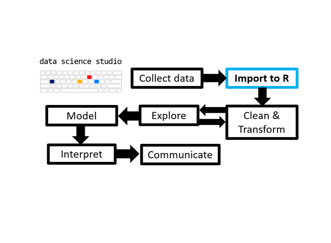
As the second post in the Scientist’s Guide to R series (click here for the 1st post), this post will goes into the first step of the data analysis with R process: importing your data from a variety of common “flat file” sources (.csv, .txt, .xlsx, etc).
2 Introduction
So you’ve spent weeks/months/years conducting a carefully planned research project and collected a bunch of data, and want to know how the study turned out using the advanced functionality of R? The first things you will need to do are:
i) Install R & R studio. Install R using this link. The R studio integrated development environment (IDE) is available here (R studio is not necessary to use R but it is strongly recommended). For instructions on using R studio, see these videos.
ii) install and load R add-on packages.
iii) import your data.
After you’ve installed R studio, read on for a brief explanation of how to install and load R packages. These additional packages greatly expand the functionality of R (e.g. allow you to build webpages like this blog using the blogdown package), making it much easier to learn and use. While there are many different ways to do things using R, this guide will cover the ways I have found in practice to have the right balance of effectiveness, efficiency, and accessibility/transparency. There are many excellent books and online resources for those wanting to learn more about alternative methods. However, to avoid confusing those attempting to learn data analysis with R for the 1st time, the scope of these tutorials will be limited to recommended methods only.
After explaining how to install and load R packages, this post will cover how to easily import data from a variety of common sources ranging from comma-separated-variable (.csv) files, to excel spreadsheets, and fixed width files.
3 Installing and Loading R Packages
Installing & loading packages into R is a very straightforward process. For packages hosted on CRAN (which is where the “official” versions of most R packages reside), simply run the following:
#To include comments in R (like this), begin the comment with "#", which will tell R
#to treat the following info as a comment and not try to run it as live R code.

#installation command
install.packages("package_name") #replace "package_name" with the name of the package
# you want to install

#load the package when you want to use it using the base R library() function
library(package_name) #replace "package_name" with the name of the package
#you've installed and want to use

# for example, some of the functions I recommend below for importing data use
# the readr package, which is part of the tidyverse suite of pacakges:

install.packages("readr") #replace "package_name" with the name of the package

library(readr)

#or if you want all of the tidyverse packages (which we will be using throughout this guide)
install.packages("tidyverse")

library(tidyverse) #loads readr along with other helpful packages, like ggplot2 for graphing.
For packages hosted on GitHub, which are typically in development, the process is slightly more complicated but still requires only couple of lines of code:
#1. first install and load the devtools package

#install devtools from CRAN
install.packages("devtools")

#load the devtools package
library(devtools)

#2. install the package of interest from its github repository using
# the install_github function()

install_github("repository_name/package_name")

# For example, to get the development version of the tidyr package,
# which contains excellent new functions for converting between the long and wide
# forms of data (there will be a later post on this), you would run:

install_github("tidyverse/tidyr") #contains more flexible
# pivoting functions than the CRAN version of tidyr.

# Packages installed from GitHub can then also be loaded using the library() function
# and the package name only:

library(tidyr)

#N.B. If you are using R studio, you can also install packages from CRAN
# by clicking on the packages tab of the lower right panel and clicking the "Install" button
4 How to Get Your Data Into R
Getting your data into R is also easy. Commands and packages specific to different data sources are listed below:
4.1 Comma Delimited (.csv) Files
CSV files are the most common type of data file you’ll encounter as a data analyst. These can be imported using the read_csv() function from the readr package.
#using the readr package:
library(readr)

read_csv("directory_path/filename.csv") #e.g. C:/Users/your_name/Desktop/documents/data.csv

# If you want to use the data after importing it, assign it to be stored in an object using
# the assignment operator: "<-"

data <- read_csv("directory_path/filename.csv")

# N.B. If you are using R studio, you can use the keyboard shortcut
# ["alt" + "-"] to insert "<-"

# you can then examine the data by simply running the assigned name

data

# or clicking on it in the "environment" window in R studio (by default it is
# in the top right panel)
4.2 Tab Delimited (.txt) Files
library(readr)

data <- read_tsv("directory_path/filename.txt")

#yes, it is that easy ;)
4.3 Files With Other Delimiting Characters (also .txt)
The read_csv() and read_tsv() functions are actually convienience wrappers for the workhorse function of the readr package, read_delim(), which can be used to read in data files with any delimiting character (e.g. “-”, “$”, etc.). This is only slightly more complicated, in that you have to specify what the delimiting character is using the delim argument.
library(readr)

data <- read_delim("directory_path/filename.txt", delim = "|")
# specify the file path/name.txt and the delimiting character,
# whatever it happens to be for your data file
4.4 Microsoft Excel Files (.xlsx, .xls)
Excel files are fairly easy to import using the readxl package. Since these files may contain several speadsheets, you also have to specify the sheet that you want to use… unless it is the first one, which is assumed by default.
library(readxl)

# If you want the first sheet then you can just specify the path
data <- read_excel(path = "path/file.xlsx")

# If you want a different sheet then you have to specify which one using the sheet argument

data <- read_excel(path = "path/file.xlsx",
                   sheet = "sheet_name")

# Using the excel_sheets helper function makes things easier by showing you what the names
# of each sheet are in the excel file.
excel_sheets("path/file.xlsx")

# You can also specify the sheet using an integer
data <- read_excel(path = "path/file.xlsx",
                   sheet = 2) #to get the 2nd sheet
4.5 Files from SPSS, SAS, or Stata
If you’ve recently switched from working in SPSS, SAS, or Stata (or are collaborating with someone who uses these programs), you can also easily import your existing SPSS or SAS data files directly into R using the haven package.
library(haven)

#SAS files
data <- read_sas("file_name.sas7bdat") #if the file is in your working directory
#otherwise specify the file path as well, e.g. "path/file_name.sas7bdat"

#SPSS files
data <- read_sav("file_name.sav")

#Stata files
data <- read_dta("file_name.dta")
4.6 Fixed Width Files (.txt, .gz, .bz2, .xz, .zip, etc.)
Fixed width files are a less common type of data source where the values are separated not by tabs or specific characters but a set amount of white/empty space other than a tab. These can be loaded using the read_fwf() function in readr.
library(readr)

# For these fixed width files, you can specify column positions (i.e. breaks between values)
# in multiple ways. See https://readr.tidyverse.org/reference/read_fwf.html,
# which I used to obtain templates of the commands below, for further details.

# The main arguments you need to include are file = the file path/name.extension,
# col_positions, and col_names().

# the col_positions argument is different from the others we've see so far (e.g. delim)
# in that it is primarily intended to be used by specifying a call to another function,
# such as fwf_empty (see below), which tells read_fwf() how you want to specify the columns.
# some options are:

# 1. Guess based on position of empty columns using the fwf_empty helper function
# as an argument(easiest):

file_path <- c("directory_path/filename.txt") #store the file path/name as "file_path"

data <- read_fwf(file = file_path,
                 col_positions = fwf_empty(file_path,
                                           col_names = c("col_1", "col_2", "col_3"))
                 #replace the above labels with column names you want to use.
                 #note that col_names is an argument supplied to the fwf_empty helper function
                 #which is then passed along to the read_fwf function.

# 2. Using a vector of field widths (a bit more tedious) with
# the fwf_widths() helper function:

data <- read_fwf(file = file_path,
                 col_positions = fwf_widths(c(10, 7, 19, 290),
                 #replace the above with values appropriate to your data
                           col_names = c("col_1", "col_2", "col_3"))

# 3. Specifying starting and ending positions of the columns with paired vectors
# using the fwf_positions() helper function

read_fwf(file = file_path,
         fwf_positions(start = c(1, 50), #which positions do the columns start at
                       end = c(25, 75), #which positions do the columns end at
                       col_names = c("col_1", "col_2"))) #list of column names

# 4. Using named arguments for starting and ending positions with
# the fwf_cols() helper function:

read_fwf(file = file_path,
         col_positions = fwf_cols(name = c(1, 10),
                                  birthdate = c(20, 50),
                                  age = c(60, 63)))

# 5. Via named arguments and column widths, also using the fwf_cols helper function:

read_fwf(file = file_path,
         fwf_cols(subject_id = 15,
         #e.g. the subject_id column contains data in the 1st 15 characters of each row
                  test_score = 20))
4.7 html/xml files
Those who need to scrape data from the web for their research can use the rvest and XML packages. Since this is not what most experimental scientists (at least among the many I’ve had the pleasure of meeting) will need to do, I have only provided the necessary functions below without a detailed explanation. See this blog post for further details.
#HTML pages
library(rvest)

#store the url
url <- c("http://www.webpagename.com")

#read in the html data
web_page <- read_html(url)

#extract the html info for the target table
web_page_table <- html_nodes(web_page, "table")

#parse the html table info into a data set that you can use in R
data <- html_table(web_page_table, fill = TRUE)

#XML
library(XML)

#read in the html data
data <- readHTMLTable(url)
4.8 JavaScript Object Notation (JSON) Files
JSON files are way of storing JavaScript objects as text that can easily be imported in to R using the fromJSON() function from the jsonlite package. Science trainees are unlikely to encounter this type of data unless they are working with web sources, e.g. twitter. See this link for an accessible overview.
library(jsonlite)
r_bloggers_data <- fromJSON("~/Desktop/r-bloggers.json")4.10 Notes
Exporting data is also easy and will be covered in a later post. E.g. for readr functions this is usually done via the appropriately named write_ functions, like write_csv().
By default, the above readr functions will assume that the first row of your data file contains the variable names. For these functions, you can disable this by setting the col_names argument to FALSE, or you can provide a string/character vector of names to use instead by setting col_names to the name of the string vector (see the next post for more on data vectors).
Arguments to a function can either be specified by name (which I have done here for the sake of transparency) or by position to save some typing. E.g.
read_fwf(file_path, fwf_cols(subject_id = 15, test_score = 20))is equivalent to the read_fwf syntax I provided above with argument names specified. There will be more on this in the next section of the blog.An R package only needs to be loaded once in an R session for the functions it contains to be available for use throughout the same session.
There are also ways to import data from relational databases using SQL syntax. However, these methods go beyond the scope of this blog series since they are not relevant to most academic researchers and may be covered in the distant future if/when I write a second volume on R for machine learning and data science. An introduction to importing data from these sources can be found here. Those who are interested in starting to learn SQL (e.g. for work) would benefit from the free Introduction to SQL for Data Science course provided by datacamp.com, which is where I started learning how to use SQL.
Users working with large flat files (> 100 MB) may want to consider the vroom function in the vroom package or fread function in the data.table package instead of readr to import their data. You could use these for flat files of any size, but the speed difference probably won’t really be noticable for smaller files.
Thank you for reading and I welcome any suggestions for future posts, comments or other feedback you might have. Feedback from beginners and science students/trainees (or with them in mind) is especially helpful in the interest of making this guide even better for them.
This blog is something I do as a volunteer in my free time. If you’ve found it helpful and want to give back, coffee donations would be appreciated.