- 1 TL;DR
- 2 Introduction
- 3 Basic Calculations
- 4 Logical Operators
- 5 Object Assignment
- 6 Basic Summary Statistics
- 7 Data Structures and Object Assignment
- 8 Random Numbers and Sampling
- 9 Functions for Describing the Structural Information of Data Objects
- 10 The Global Environment
- 11 The Working Directory
- 12 Projects
- 13 Useful Keyboard Shortcuts (for R studio users)
1 TL;DR
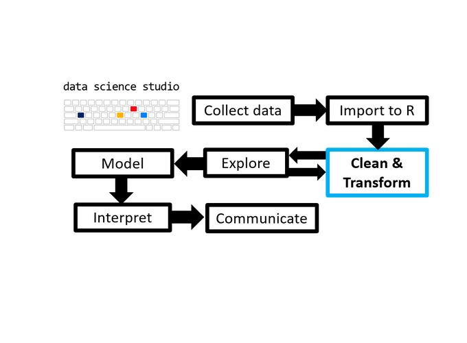
As the third post in the Scientist’s Guide to R series (click here for the 1st post), we advance to the brink of the next major stage of the data analysis with R process: cleaning and transforming data. However, before we can clean or transform anything we will need to know how to do a few basic things and familiarize ourselves with some common data structures in R, which are the topics of this post.
2 Introduction
You’ve managed to import your data and are wondering what to do next? The way in which you should proceed will critically depend upon the structure of your data, but before we get there you need to know which sorts of things you can do in R. Accordingly, this post will introduce you to some basic operations and data structures. There is a lot of content here so feel free to skip sections you are already familiar with. If this is all new you should take the time to read it since we will continue building upon this foundation as we progress to more advanced topics. You need to understand how data are represented by R before you start manipulating those representations.
3 Basic Calculations
Like any decent data analysis software, R can perform common mathematical and logical operations, as simply as you probably expect them to be.
#Basic calculations#####
5+6 #addition

89-28 #subtraction

7000*10 #multiplication

25/5 #division

2^20 #^ means to the power of

exp(8) #exponential

37 %% 2 #modulus. Returns the remainder after division.
4 Logical Operators
Also very straightforward. These are mostly useful when selecting subsets of data or programming.
#use double equality symbols to check for equality since "=" is reserved for
#assignment or value specification

1 == 1 #LHS is equal to RHS

1 != 1 #LHS is not equal to RHS

10 > 8 #LHS greater than RHS

10 >= 8 #LHS greater than or equal to RHS

10 < 8 #LHS less than RHS

5 <= 5 #LHS less than or equal to RHS

(1 > 3) & (10 > 3) #are both 1 and 10 greater than 3?

(1 > 3) | (10 > 3) #is 1 or 10 greater than 3?

#see https://www.statmethods.net/management/operators.html for more examples.
5 Object Assignment
To save some values (or virtually anything else) to use again later you assign them to a variable. This can be done in R using either “<-” or “=”, but “<-” is typically recommended. See here for the subtleties, e.g. “=” sometimes fails when you wouldn’t expect it to, but “<-” typically does not. R studio also provides a handy keyboard shortcut for inserting “<-”: [Alt] & [-]
x <- 27 #this stores whatever is on the RHS in the arbitrarily named variable on the LHS
x #to print it to the console, just call the variable.## [1] 27#you can assign something to a variable and print it at the same time by wrapping it in parentheses
(y <- 900)## [1] 900#although doing so is uncommon, the use of arrows for assignment also enables
#you to assign things in the opposite direction, from left to right. Arrows also
#make it obvious which side is being assigned to which side of the operator
90 -> z
z## [1] 90#to remove a variable from your environment use the rm() function
rm(x)
#assigning something to a variable that is already in use will overwrite the variable
y <- 8
y## [1] 8#the only naming conventions are that a name should not begin with a
#number, and you should avoid using names that already exist as functions in R
#or special characters, e.g.:
1.m <- 7 #starting a variable name with a number produces an error
TRUE <- 9 #TRUE is a reserved keyword for the logical statement true, also results in an error
mean <- 99 #here I assign the number 99 to the same name as the mean function
#this is probably not what you want since it makes calling mean ambiguous.
mean
rm(mean)
#to check if a name is already reserved for something else, just try to look up
#the help page for it using ?name
?mean
#since pretty much anything can be assigned to a variable, you can also chain assignment operations
(y <- 900)
(z <- y <- 900) #store the RHS in 2 separate variables, called y and z
#usually you would store something slightly different in each of them, e.g. a
#modification of the 1st variable is stored in a 2nd variable
z <- y + 10
z6 Basic Summary Statistics
R makes it incredibly easy to get simple summary statistics for numeric variables. So while we won’t dive too deeply into exploratory data analysis until later in the blog series we’ll get our toes wet here.
#R also provides a set of basic functions for conducting common summary
#statistic calculations
x <- c(0:10)

sum(x) #obtain the sum of the sequence of numbers from 1 to 100## [1] 55mean(x) #mean## [1] 5sd(x) #standard deviation## [1] 3.316625median(x) #a shortcut for the 50th percentile AKA the median## [1] 5min(x) #the minimum## [1] 0max(x) #the maximum## [1] 107 Data Structures and Object Assignment
Most of the things you will do in R operate upon a variety of objects.
The common R data structures are:
Vectors = a one-dimensional array of data elements/values
Factors = R’s way of representing vectors as categorical variables for statistical testing and data visualization purposes.
Matrices = a two-dimensional array of vectors arranged in columns and rows. All data elements are typically of the same class. Columns are rows are numbered by position from left to right (columns) and top to bottom (rows).
Data Frames = Also a 2D array but columns can be different classes. These are the most common data structure in R.
Tibbles = an enhanced version of the data frame with improved display characteristics. Tibbles have gained popularity as the tidyverse has become more prominent over the past few years.
Lists: a list of arbitrary objects, more flexible than data frames but less intuitive to work with. Lists elements can consist of multiple different data types, including the output of statistical tests and even entire data frames. Lists are a more advanced topic so they won’t be covered further for the time being. If you want to learn more about them now see this video.
Arrays: If you want to work with matrices that have more than 2 dimensions (remember that a matrix is a 2D array), checkout the array function. Arrays with more than 2 dimensions are not commonly used for the analysis of most forms of experimental data (e.g. I’ve never needed them), so I won’t be covering them in this blog series. Those who are interested in learning more about them can find a brief intro here. A more detailed treatment is provided in section 5 of the official R introductory manual
N.B. One of the most important functions that base R provides is str(), which enables you to inspect the structure of any object.
7.1 Numeric and Character Vectors
#A vector is a one-dimensional array of numerical values or character strings.
#You can create one using the c() function in R, e.g.:

c(1, 3, 4, 5, 6)## [1] 1 3 4 5 6#to save this vector for future use, you assign it to a variable using either "=" or "<-"
#it is generally recommended to use "<-" for assignment instead of "=", although either will work
#By wrapping the vector in str(), you gain structural information
str(c(1, 3, 4, 5, 6)) #a numeric vector of length 5, with values shown## num [1:5] 1 3 4 5 6c(1:100) #all numbers between a range can be specified using number:number## [1] 1 2 3 4 5 6 7 8 9 10 11 12 13 14 15 16 17 18
## [19] 19 20 21 22 23 24 25 26 27 28 29 30 31 32 33 34 35 36
## [37] 37 38 39 40 41 42 43 44 45 46 47 48 49 50 51 52 53 54
## [55] 55 56 57 58 59 60 61 62 63 64 65 66 67 68 69 70 71 72
## [73] 73 74 75 76 77 78 79 80 81 82 83 84 85 86 87 88 89 90
## [91] 91 92 93 94 95 96 97 98 99 100str(c(1:100)) #a numeric vector of length 100, with the 1st 10 values shown## int [1:100] 1 2 3 4 5 6 7 8 9 10 ...c("a", "b", "c") #character values/strings need to be quoted to be parsed correctly## [1] "a" "b" "c"#anything entered in quotation marks is read text/character, and if at least 1
#element is quoted, all elements of a vector are coerced to string format
c("1", 2, "3") #prints as a character vector## [1] "1" "2" "3"#if a string vector contains only numbers, you can reclassify it as numeric
#using as.numeric()
as.numeric(c("1", 2, "3")) #now it prints as a numeric vector## [1] 1 2 3str(c("a", "b", "c")) #str tells us that this is a character vector of length 3## chr [1:3] "a" "b" "c"c("apples", "bananas", "cherries") #each entry is in quotations and separated by a comma## [1] "apples" "bananas" "cherries"str(c("apples", "bananas", "cherries")) #also a character vector of length 3## chr [1:3] "apples" "bananas" "cherries"c_vect <- letters[seq(from = 1, to = 26)] #letters[] lets you quickly create a character vector of letters
#There are 2 subclasses of numeric vector:
#"integer", which contains only whole numbers, and "double"(also simply called
#numeric; both labels refer to the same thing), which has both integer and
#decimal components
#the class function returns the class of an object. see ?class for more info.
x <- c(1, 3, 4, 5, 6)
class(x) #by default, both integers and doubles are classified as "numeric"## [1] "numeric"x <- as.integer(x) #you can coerce a vector into a different class, if it is reasonable to do so.
class(x) #now R reads the number list as an integer vector## [1] "integer"#to conduct a logical test to see if an object is a particular class use
#is.[class] (insert the class name), e.g.
is.integer(x)## [1] TRUE7.2 Logical Vectors
l <- c(TRUE, FALSE, TRUE, TRUE, FALSE, TRUE) #logical vector
l <- c(T, F, T, T, F, T) #equivalent short hand version
class(l)
## [1] "logical"#"TRUE" and "FALSE", which may be abbreviated as "T" and "F", are also read by R as 1 and 0 respectively.
#this conveniently enables you to obtain the total number of TRUE elements using the sum() function
sum(l)## [1] 4#you can also get the proportion of TRUE values using the mean function
mean(l)## [1] 0.6666667#both of these are very useful when conducting logical tests of a vector to see
#how many elements match the specified criteria, e.g.:
x <- c(1:10, 100:130)
x < 50 #returns a logical vector with True corresponding to elements matching the logical test, ## [1] TRUE TRUE TRUE TRUE TRUE TRUE TRUE TRUE TRUE TRUE FALSE FALSE
## [13] FALSE FALSE FALSE FALSE FALSE FALSE FALSE FALSE FALSE FALSE FALSE FALSE
## [25] FALSE FALSE FALSE FALSE FALSE FALSE FALSE FALSE FALSE FALSE FALSE FALSE
## [37] FALSE FALSE FALSE FALSE FALSE#in this case that the value is less than 50
sum(x < 50) #how many values in x are less than 50## [1] 10mean(x < 50) #what proportion of the values in x are less than 50## [1] 0.2439024#using modulus 2 (divide by 2 and return the remainder) can tell you which
#elements of a numeric vector are odd or even, which is most useful for programming.
(x %% 2) == 0 #even values in x = TRUE## [1] FALSE TRUE FALSE TRUE FALSE TRUE FALSE TRUE FALSE TRUE TRUE FALSE
## [13] TRUE FALSE TRUE FALSE TRUE FALSE TRUE FALSE TRUE FALSE TRUE FALSE
## [25] TRUE FALSE TRUE FALSE TRUE FALSE TRUE FALSE TRUE FALSE TRUE FALSE
## [37] TRUE FALSE TRUE FALSE TRUE(x %% 2) == 1 #odd values in x = TRUE## [1] TRUE FALSE TRUE FALSE TRUE FALSE TRUE FALSE TRUE FALSE FALSE TRUE
## [13] FALSE TRUE FALSE TRUE FALSE TRUE FALSE TRUE FALSE TRUE FALSE TRUE
## [25] FALSE TRUE FALSE TRUE FALSE TRUE FALSE TRUE FALSE TRUE FALSE TRUE
## [37] FALSE TRUE FALSE TRUE FALSE#you can do similar tests with character vectors
c_vect <- c("a", "b", "a", "c", "d")
mean(c_vect == "a") #how many elements of c_vect are "a"## [1] 0.4sum(c_vect == "a") #what proportion of the elements of c_vect are "a"## [1] 2#logical tests are also used to subset or filter data, as demonstrated later on...7.3 Factors
#Factors are a modified form of either a characeter or numeric vector which
#facilitates their use as categorical variables. You can create a factor in R
#using either the factor() function, or by reclassifying another vector type
#using as.factor()

x <- c(1:3, 1:3, 1:3)
as.factor(x) ## [1] 1 2 3 1 2 3 1 2 3
## Levels: 1 2 3#Note the addition of levels to the output. What as.factor does is assign each
#unique value of the vector to a level of the factor. Under the hood this also
#involves constructing a set of 0/1 dummy variables for each level of the
#factor, which are needed to fit some models, like linear regession models (but
#don't worry about this, because R will do it for you automatically).
#using the factor() function instead allows you to assign labels to the levels
#you can also specify whether or not the factor is ordered
factor(x, levels = c(1, 2, 3), labels = c("one", "two", "three"), ordered = TRUE)## [1] one two three one two three one two three
## Levels: one < two < three7.4 Matrices
#the matrix() function allows you to create a matrix

#create an empty matrix with row and column dimensions specified using nrow and
#ncol arguments. This can be useful if you plan to fill it in later (e.g. when
#writing loops).
mat1 <- matrix(nrow = 100, ncol = 10)

str(mat1) #view the structure of the new matrix## logi [1:100, 1:10] NA NA NA NA NA NA ...#take a vector and distribute the values into 2 columns with 20 rows each
matrix(data = c(1:40), nrow = 20, ncol = 2) ## [,1] [,2]
## [1,] 1 21
## [2,] 2 22
## [3,] 3 23
## [4,] 4 24
## [5,] 5 25
## [6,] 6 26
## [7,] 7 27
## [8,] 8 28
## [9,] 9 29
## [10,] 10 30
## [11,] 11 31
## [12,] 12 32
## [13,] 13 33
## [14,] 14 34
## [15,] 15 35
## [16,] 16 36
## [17,] 17 37
## [18,] 18 38
## [19,] 19 39
## [20,] 20 40#you can combine vectors into a matrix using cbind(vector1, vector2) or
#rbind(vector1, vector2) depending on whether you want to combine elements as
#row vectors or column vectors. each must be the same lenght, otherwise some
#elements will be coded as NA for the shorter vector
x1 <- c(1:50)
x2 <- c(51:100)
x3 <- c(1:10)
(mat1 <- cbind(x1, x2)) #combined by column## x1 x2
## [1,] 1 51
## [2,] 2 52
## [3,] 3 53
## [4,] 4 54
## [5,] 5 55
## [6,] 6 56
## [7,] 7 57
## [8,] 8 58
## [9,] 9 59
## [10,] 10 60
## [11,] 11 61
## [12,] 12 62
## [13,] 13 63
## [14,] 14 64
## [15,] 15 65
## [16,] 16 66
## [17,] 17 67
## [18,] 18 68
## [19,] 19 69
## [20,] 20 70
## [21,] 21 71
## [22,] 22 72
## [23,] 23 73
## [24,] 24 74
## [25,] 25 75
## [26,] 26 76
## [27,] 27 77
## [28,] 28 78
## [29,] 29 79
## [30,] 30 80
## [31,] 31 81
## [32,] 32 82
## [33,] 33 83
## [34,] 34 84
## [35,] 35 85
## [36,] 36 86
## [37,] 37 87
## [38,] 38 88
## [39,] 39 89
## [40,] 40 90
## [41,] 41 91
## [42,] 42 92
## [43,] 43 93
## [44,] 44 94
## [45,] 45 95
## [46,] 46 96
## [47,] 47 97
## [48,] 48 98
## [49,] 49 99
## [50,] 50 100class(mat1)## [1] "matrix" "array"(mat2 <- rbind(x1, x2)) #combined by row## [,1] [,2] [,3] [,4] [,5] [,6] [,7] [,8] [,9] [,10] [,11] [,12] [,13] [,14]
## x1 1 2 3 4 5 6 7 8 9 10 11 12 13 14
## x2 51 52 53 54 55 56 57 58 59 60 61 62 63 64
## [,15] [,16] [,17] [,18] [,19] [,20] [,21] [,22] [,23] [,24] [,25] [,26]
## x1 15 16 17 18 19 20 21 22 23 24 25 26
## x2 65 66 67 68 69 70 71 72 73 74 75 76
## [,27] [,28] [,29] [,30] [,31] [,32] [,33] [,34] [,35] [,36] [,37] [,38]
## x1 27 28 29 30 31 32 33 34 35 36 37 38
## x2 77 78 79 80 81 82 83 84 85 86 87 88
## [,39] [,40] [,41] [,42] [,43] [,44] [,45] [,46] [,47] [,48] [,49] [,50]
## x1 39 40 41 42 43 44 45 46 47 48 49 50
## x2 89 90 91 92 93 94 95 96 97 98 99 100class(mat2)## [1] "matrix" "array"#combining vecotrs of unequal length produces NAs for the extra indices of the
#longer one
#common matrix operations work as expected with matrix objects in R
t(mat1) #transposition## [,1] [,2] [,3] [,4] [,5] [,6] [,7] [,8] [,9] [,10] [,11] [,12] [,13] [,14]
## x1 1 2 3 4 5 6 7 8 9 10 11 12 13 14
## x2 51 52 53 54 55 56 57 58 59 60 61 62 63 64
## [,15] [,16] [,17] [,18] [,19] [,20] [,21] [,22] [,23] [,24] [,25] [,26]
## x1 15 16 17 18 19 20 21 22 23 24 25 26
## x2 65 66 67 68 69 70 71 72 73 74 75 76
## [,27] [,28] [,29] [,30] [,31] [,32] [,33] [,34] [,35] [,36] [,37] [,38]
## x1 27 28 29 30 31 32 33 34 35 36 37 38
## x2 77 78 79 80 81 82 83 84 85 86 87 88
## [,39] [,40] [,41] [,42] [,43] [,44] [,45] [,46] [,47] [,48] [,49] [,50]
## x1 39 40 41 42 43 44 45 46 47 48 49 50
## x2 89 90 91 92 93 94 95 96 97 98 99 100t(mat1) + mat2 #addition (both matrices need to have the same dimensions)## [,1] [,2] [,3] [,4] [,5] [,6] [,7] [,8] [,9] [,10] [,11] [,12] [,13] [,14]
## x1 2 4 6 8 10 12 14 16 18 20 22 24 26 28
## x2 102 104 106 108 110 112 114 116 118 120 122 124 126 128
## [,15] [,16] [,17] [,18] [,19] [,20] [,21] [,22] [,23] [,24] [,25] [,26]
## x1 30 32 34 36 38 40 42 44 46 48 50 52
## x2 130 132 134 136 138 140 142 144 146 148 150 152
## [,27] [,28] [,29] [,30] [,31] [,32] [,33] [,34] [,35] [,36] [,37] [,38]
## x1 54 56 58 60 62 64 66 68 70 72 74 76
## x2 154 156 158 160 162 164 166 168 170 172 174 176
## [,39] [,40] [,41] [,42] [,43] [,44] [,45] [,46] [,47] [,48] [,49] [,50]
## x1 78 80 82 84 86 88 90 92 94 96 98 100
## x2 178 180 182 184 186 188 190 192 194 196 198 200t(mat1) - mat2 #subtraction## [,1] [,2] [,3] [,4] [,5] [,6] [,7] [,8] [,9] [,10] [,11] [,12] [,13] [,14]
## x1 0 0 0 0 0 0 0 0 0 0 0 0 0 0
## x2 0 0 0 0 0 0 0 0 0 0 0 0 0 0
## [,15] [,16] [,17] [,18] [,19] [,20] [,21] [,22] [,23] [,24] [,25] [,26]
## x1 0 0 0 0 0 0 0 0 0 0 0 0
## x2 0 0 0 0 0 0 0 0 0 0 0 0
## [,27] [,28] [,29] [,30] [,31] [,32] [,33] [,34] [,35] [,36] [,37] [,38]
## x1 0 0 0 0 0 0 0 0 0 0 0 0
## x2 0 0 0 0 0 0 0 0 0 0 0 0
## [,39] [,40] [,41] [,42] [,43] [,44] [,45] [,46] [,47] [,48] [,49] [,50]
## x1 0 0 0 0 0 0 0 0 0 0 0 0
## x2 0 0 0 0 0 0 0 0 0 0 0 0t(mat1) * mat2 #multiplication## [,1] [,2] [,3] [,4] [,5] [,6] [,7] [,8] [,9] [,10] [,11] [,12] [,13] [,14]
## x1 1 4 9 16 25 36 49 64 81 100 121 144 169 196
## x2 2601 2704 2809 2916 3025 3136 3249 3364 3481 3600 3721 3844 3969 4096
## [,15] [,16] [,17] [,18] [,19] [,20] [,21] [,22] [,23] [,24] [,25] [,26]
## x1 225 256 289 324 361 400 441 484 529 576 625 676
## x2 4225 4356 4489 4624 4761 4900 5041 5184 5329 5476 5625 5776
## [,27] [,28] [,29] [,30] [,31] [,32] [,33] [,34] [,35] [,36] [,37] [,38]
## x1 729 784 841 900 961 1024 1089 1156 1225 1296 1369 1444
## x2 5929 6084 6241 6400 6561 6724 6889 7056 7225 7396 7569 7744
## [,39] [,40] [,41] [,42] [,43] [,44] [,45] [,46] [,47] [,48] [,49] [,50]
## x1 1521 1600 1681 1764 1849 1936 2025 2116 2209 2304 2401 2500
## x2 7921 8100 8281 8464 8649 8836 9025 9216 9409 9604 9801 10000t(mat1) / mat2 #division## [,1] [,2] [,3] [,4] [,5] [,6] [,7] [,8] [,9] [,10] [,11] [,12] [,13] [,14]
## x1 1 1 1 1 1 1 1 1 1 1 1 1 1 1
## x2 1 1 1 1 1 1 1 1 1 1 1 1 1 1
## [,15] [,16] [,17] [,18] [,19] [,20] [,21] [,22] [,23] [,24] [,25] [,26]
## x1 1 1 1 1 1 1 1 1 1 1 1 1
## x2 1 1 1 1 1 1 1 1 1 1 1 1
## [,27] [,28] [,29] [,30] [,31] [,32] [,33] [,34] [,35] [,36] [,37] [,38]
## x1 1 1 1 1 1 1 1 1 1 1 1 1
## x2 1 1 1 1 1 1 1 1 1 1 1 1
## [,39] [,40] [,41] [,42] [,43] [,44] [,45] [,46] [,47] [,48] [,49] [,50]
## x1 1 1 1 1 1 1 1 1 1 1 1 1
## x2 1 1 1 1 1 1 1 1 1 1 1 17.5 Dataframes
#data frames can be constructed using the dataframe function,
#or by converting a combination of vectors/matrix using as.data.frame()
x <- cbind(sample(1:6), rep(c("a", "b", "c"), 2)) #create a 2-column

class(x) #a matrix
## [1] "matrix" "array"#if names are not associated with the columns the variables are labelled using
#V[index]
df <- as.data.frame(x)
df## V1 V2
## 1 4 a
## 2 1 b
## 3 2 c
## 4 5 a
## 5 6 b
## 6 3 cclass(df) #now a data frame## [1] "data.frame"df <- as.data.frame(x)
names(df) <- c("var_1", "var_2") #change column names using the names() function
str(df)## 'data.frame': 6 obs. of 2 variables:
## $ var_1: chr "4" "1" "2" "5" ...
## $ var_2: chr "a" "b" "c" "a" ...#create the data frame directly and specify names
df <- data.frame("var_1" = c(sample(1:6, 6)),
"var_2" = rep(c("a", "b", "c"), 2))
str(df)## 'data.frame': 6 obs. of 2 variables:
## $ var_1: int 2 1 4 6 5 3
## $ var_2: chr "a" "b" "c" "a" ...#if you don't want strings to be converted to factors automatically, set
#stringsAsFactors = FALSE
df <- data.frame("var_1" = c(sample(1:6, 6)),
"var_2" = rep(c("a", "b", "c"), 2),
stringsAsFactors = FALSE) 7.6 Tibbles
#load the tidyverse packages, which contain the tibble and as_tibble functions
library(tidyverse)
## -- Attaching packages --------------------------------------- tidyverse 1.3.0 --## v ggplot2 3.3.3 v purrr 0.3.4
## v tibble 3.1.1 v dplyr 1.0.2
## v tidyr 1.1.2 v stringr 1.4.0
## v readr 1.4.0 v forcats 0.5.0## Warning: package 'ggplot2' was built under R version 4.0.5## Warning: package 'tibble' was built under R version 4.0.5## -- Conflicts ------------------------------------------ tidyverse_conflicts() --
## x dplyr::filter() masks stats::filter()
## x dplyr::lag() masks stats::lag()#convert a df or matrix to a tibble using as_tibble()
df <- data.frame("var_1" = c(sample(1:6, 6)),
"var_2" = rep(c("a", "b", "c"), 2))
tbl1 <- as_tibble(df)
tbl1 #printout also tells you the dimensions and class of each column## # A tibble: 6 x 2
## var_1 var_2
## <int> <chr>
## 1 2 a
## 2 6 b
## 3 1 c
## 4 5 a
## 5 4 b
## 6 3 c#When creating a tibble, strings are not automatically converted to factors.
#This is better from a data manipulation standpoint, which will be covered in a
#future post on working with strings
tbl1 <- tibble("var_1" = c(sample(1:6, 6)),
"var_2" = rep(c("a", "b", "c"), 2))
tbl1## # A tibble: 6 x 2
## var_1 var_2
## <int> <chr>
## 1 6 a
## 2 5 b
## 3 1 c
## 4 3 a
## 5 2 b
## 6 4 c8 Random Numbers and Sampling
#sampling

#obtain a random sample 6 numbers with values ranging between 1 and 40 without replacement
sample(1:40, 6, replace=F) ## [1] 6 12 24 15 19 34x <- c(1:30)
x## [1] 1 2 3 4 5 6 7 8 9 10 11 12 13 14 15 16 17 18 19 20 21 22 23 24 25
## [26] 26 27 28 29 30v <- sample(1:200, 100, replace=T) #sample with replacement, save it in a vector called "v"
v## [1] 132 133 69 141 186 182 189 191 155 35 22 88 36 129 95 87 72 117
## [19] 143 35 136 121 51 61 157 152 81 51 78 105 60 37 43 101 22 180
## [37] 117 55 176 123 38 107 60 147 72 188 67 4 123 41 36 196 67 27
## [55] 14 152 192 182 64 106 60 185 181 16 182 168 105 167 200 18 79 140
## [73] 99 6 81 156 185 9 21 158 126 40 184 120 40 160 35 126 159 169
## [91] 145 19 166 164 2 168 118 178 29 58set.seed(seed = 934) #sets criteria for random sampling for variable creation if you want it to be repeatable
random.sample <- rnorm(1000, mean = 100, sd = 1) #create a dataset of random, normally distributed data
#generating sequences
seq(from = 1, to = 7, by = 1) #generate a sequence of numbers from 1 to 7, in 1 unit increments.## [1] 1 2 3 4 5 6 7seq(1, 7, 1) #specify arguments by position instead## [1] 1 2 3 4 5 6 7rep(1:10, each = 2)## [1] 1 1 2 2 3 3 4 4 5 5 6 6 7 7 8 8 9 9 10 10x <- c(1:12)
rep(x, each = 2) #create a numeric vector containing each element of x repeated twice## [1] 1 1 2 2 3 3 4 4 5 5 6 6 7 7 8 8 9 9 10 10 11 11 12 12rep(seq(1, 7, 1), each = 3) #repeat a sequence## [1] 1 1 1 2 2 2 3 3 3 4 4 4 5 5 5 6 6 6 7 7 7x <- seq(1, 7, 1)
rep(x, each = 3) #equivalent to the nested version## [1] 1 1 1 2 2 2 3 3 3 4 4 4 5 5 5 6 6 6 7 7 7#creating a data frame from scratch
y <- c(rnorm(n = 60, mean = 100, sd = 20), rnorm(n = 10, mean = 110, sd = 20)) #creates variable y composed of 60 random scores from a normal distribution with a mean of 100 and sd of 20, along with 10 random scores from a normal distribution with a mean of 110 and sd of 20
g <- factor(rep(seq(1, 7, 1), each = 10), labels = "g", ordered = FALSE) #groups the scores from 'y' into 7 sets (g1,g2,etc) containing 10 scores each
z <- letters[1:5]
df <- as.data.frame(cbind(y, g, z))
class(df)## [1] "data.frame"class(df$y)## [1] "character"df$y <- as.numeric(df$y) #convert to numeric
class(df$z) #check the class of variable "Z"## [1] "character"class(df$g) #check the class of variable "g"## [1] "character"9 Functions for Describing the Structural Information of Data Objects
length(c(1:100)) #number of elements in a vector = the length of the vector## [1] 100data <- mtcars #we'll use the built-in mtcars dataframe as an example again
length(data) #when used on a matrix or data frame, returns the number of columns## [1] 11nrow(data) #number of rows## [1] 32ncol(data) #number of columns## [1] 11dim(data) #returns the number of rows and columns of the object## [1] 32 11unique(data$cyl) #display the unique values of the specified variable## [1] 6 4 8#useful applications of the unique() function include making it easier to
#construct factors (since you need to know what the unique values are) and
#making it easier to identify data entry errors (to be demonstrated in a future
#post)
levels(as.factor(data$cyl)) #this is the same as unique but for factors. ## [1] "4" "6" "8"#It provides the added benefit of revealing the order of factor levels.
#show the unique values of a vector (top line)
#as well as the count of each (bottom line)
table(data$cyl) ##
## 4 6 8
## 11 7 14#of course the str() function, which we've already covered is incredibly
#versatile and informative
str(data$cyl) #the structure of a variable within a dataframe## num [1:32] 6 6 4 6 8 6 8 4 4 6 ...str(data) #the structure of a whole dataframe## 'data.frame': 32 obs. of 11 variables:
## $ mpg : num 21 21 22.8 21.4 18.7 18.1 14.3 24.4 22.8 19.2 ...
## $ cyl : num 6 6 4 6 8 6 8 4 4 6 ...
## $ disp: num 160 160 108 258 360 ...
## $ hp : num 110 110 93 110 175 105 245 62 95 123 ...
## $ drat: num 3.9 3.9 3.85 3.08 3.15 2.76 3.21 3.69 3.92 3.92 ...
## $ wt : num 2.62 2.88 2.32 3.21 3.44 ...
## $ qsec: num 16.5 17 18.6 19.4 17 ...
## $ vs : num 0 0 1 1 0 1 0 1 1 1 ...
## $ am : num 1 1 1 0 0 0 0 0 0 0 ...
## $ gear: num 4 4 4 3 3 3 3 4 4 4 ...
## $ carb: num 4 4 1 1 2 1 4 2 2 4 ...str(table) #the structure of a function## function (..., exclude = if (useNA == "no") c(NA, NaN), useNA = c("no",
## "ifany", "always"), dnn = list.names(...), deparse.level = 1)#the tidyverse alternative to str is the glimpse function(), which is
#specialized for displaying the structural info of dataframes and tibbles,
#providing a slightly nicer printout, and enabling you to peak at the structure
#of the data in the middle of a series of "piped" or "chained" operations
#without interrupting the sequence (more on this in the next post).
library(tidyverse)
df <- data.frame("var_1" = c(sample(1:6, 6)),
"var_2" = rep(c("a", "b", "c"), 2))
glimpse(df)## Rows: 6
## Columns: 2
## $ var_1 <int> 3, 5, 4, 1, 2, 6
## $ var_2 <chr> "a", "b", "c", "a", "b", "c"10 The Global Environment
The functions you use in R operate within what is called the global environment, which consists of the functions and other objects that you have loaded in the current R session (this is what happens you load a package with the library function), as well as any variables, data objects, or functions you have created during the session.
#to get a list of the objects in your global environment, use the ls() function
ls()
## [1] "c_vect" "data" "df" "g"
## [5] "l" "mat1" "mat2" "random.sample"
## [9] "tbl1" "v" "x" "x1"
## [13] "x2" "x3" "y" "z"11 The Working Directory
R is always connected to a specific folder on your computer called the working directory, which is the default path for loading/importing files or saving/exporting them
#to view your current working directory, use the getwd() function, or you can
#click on the "files" tab in the bottom right pane of R studio.
getwd()

#you can change your working directory using the setwd() function,
#or you can use the "set working directory' menu under the "Session" drop down
#menu along the top of the R studio window,
#or you can just use the keyboard shortcut Ctrl + Shift + H

setwd("C:/Users/CPH/Documents/")
12 Projects
The projects feature of R studio makes it much easier to keep your work organized, and using it is strongly recommended if you are working on anything that will take longer than one or two sessions to complete.
You can create/start a project using the projects menu by clicking on this button:

You can find it in the top right corner of R studio, directly below the minimize/maximize/exit buttons. Creating (or loading) a package also sets the working directory to the project folder automatically.
13 Useful Keyboard Shortcuts (for R studio users)
One of the great benefits of using R studio are the keyboard shortcuts that speed up the coding process. Here are some I’ve found to be useful:
assignment operator <-: [Alt] + [-]
extract variable: [Ctrl] + [Alt] + [v]. Highlight some code, use this shortcut, and enter the variable name
comment lines in/out: [Ctrl] + [Shift] + [c]
reflow comments: highlight/select comments and use [Ctrl] + [Shift] + [/] to reflow/wrap them for easier reading.
reindent lines: use [Ctrl] + [i] to realign the indentation of your R code so it is easier to read.
insert code section title: [Ctrl] + [Shift] + [r]. This can also be done by starting a line with # to comment it out, and ending it with #### or —-
open/close the R script outline, which contains a list of the code sections you’ve defined using the code section titles that can be clicked on to quickly navigate through your script: [Ctrl] + [Shift] + [o]
view the definition of a function: press [F2] when the cursor is on a function name
N.B. To see all available keyboard shortcuts use [Alt] + [Shift] + [K] or click “keyboard shortcuts help” under the R studio help menu. Many of the more useful ones are also accessible under the R studio code menu.
13.2 Notes
- For more details on the data structures and operations introduced in this post, you may find the official R introductory manual or Michael Crawley’s “The R Book” helpful.
Thank you for visiting my blog. I welcome any suggestions for future posts, comments or other feedback you might have. Feedback from beginners and science students/trainees (or with them in mind) is especially helpful in the interest of making this guide even better for them.
This blog is something I do as a volunteer in my free time. If you’ve found it helpful and want to give back, coffee donations would be appreciated.