1 TL;DR

Out in the real world you may often find yourself working with data from multiple sources. It will probably be stored in separate files and you’ll need to combine them before you can attempt to answer any of your research questions. This post will show you how you can combine data frames using another set of dplyr functions called joins.

2 Introduction

The 6th post of the Scientist’s Guide to R series is all about using joins to combine data. While tidy data organized nicely into a single .csv or .xlsx spreadsheet may be provided to you in courses, in the real world you’ll often collect data from multiple sources often only containing one or two similar “key” columns (like subject ID #) and have to combine pieces of them to do anything interesting. This type of data is called relational data, since the datasets are related through common key column(s). Relational databases are how most data are stored in modern non-academic organizations.

Fortunately, a package we’re already familiar with from a couple of posts ago, dplyr, also has a set of functions for combining data with functions called “joins”. For this post we will cover the 6 most common joins:

1. left_join(x, y) which combines all columns in data frame x with those in data frame y but only retains rows from x.

2. right_join(x, y) also keeps all columns but operates in the opposite direction, returning only rows from y.

3. full_join(x, y) combines all columns of x with all columns of y and retains all rows from both data frames.

4. inner_join(x, y) combines all columns present in either x or y but only retains rows that are present in both data frames.

5. semi_join(x, y) returns the columns from x only and retains rows of x that are also present in y

6. anti_join(x, y) returns the columns from x only and retains rows of x that are not present in y.

A nice design feature of these functions is that their names and behaviour were inspired by analogous functions for joining data in the ubiquitous database management programming language “Stuctured Query Language” (SQL). Learning dplyr therefore also makes SQL easier to learn in the future, which will be helpful if you ever want to work with data for a living.

In case you find yourself working in an environment where only base R is available, we’ll also cover how to join data using the base R function merge().

Aside from specifying the data frames to be joined, one other thing we need to do is specify the key column(s) to be used for aligning the rows prior to joining the data.

Key columns are specified with the by argument, e.g. inner_join(x, y, by = "subject_id") adds columns of y to x for all rows where the values of the “subject_id” column (present in each data frame) match. If the name of the key column differs between the data frames, e.g. “subject_id” in x and “subj_id” in y, then you have to specify both names using by = c("subject_id" = "subj_id") so that the functions know which columns to compare.

A nice feature of the *_join() functions is that if you don’t specify the by argument they will assume that columns with the same names across x and y are key columns. This is very convenient when the columns with the same names in fact contain the same type of values.

library(gapminder) #contains the gapminder data

library(dplyr) #functions for manipulating and joining data

life_df <- gapminder %>%
  filter(year >= 1997 & year <= 2007) %>%
  group_by(continent, year) %>% 
  summarise(mean_life_expectancy = mean(lifeExp, na.rm = T)) %>% 
  filter(continent != "Asia") %>% ungroup()

pop_df <- gapminder %>% 
  filter(year >= 1997 & year <= 2007) %>%
  group_by(continent, year) %>% 
  summarise(total_population = sum(pop, na.rm = T)) %>% 
  filter(continent != "Europe") %>%
  ungroup()


gdp_df <- gapminder %>% 
  filter(year == 1997 | year == 2007) %>%
  group_by(continent, year) %>% 
  summarise(total_gdpPercap = sum(gdpPercap, na.rm = T)) %>% 
  ungroup()

life_df %>% glimpse()

## Rows: 12
## Columns: 3
## $ continent            <fct> Africa, Africa, Africa, Americas, Americas, Ameri~
## $ year                 <int> 1997, 2002, 2007, 1997, 2002, 2007, 1997, 2002, 2~
## $ mean_life_expectancy <dbl> 53.59827, 53.32523, 54.80604, 71.15048, 72.42204,~

pop_df %>% glimpse()

## Rows: 12
## Columns: 3
## $ continent        <fct> Africa, Africa, Africa, Americas, Americas, Americas,~
## $ year             <int> 1997, 2002, 2007, 1997, 2002, 2007, 1997, 2002, 2007,~
## $ total_population <dbl> 743832984, 833723916, 929539692, 796900410, 849772762~

gdp_df %>% glimpse()

## Rows: 10
## Columns: 3
## $ continent       <fct> Africa, Africa, Americas, Americas, Asia, Asia, Europe~
## $ year            <int> 1997, 2007, 1997, 2007, 1997, 2007, 1997, 2007, 1997, ~
## $ total_gdpPercap <dbl> 123695.50, 160629.70, 222232.52, 275075.79, 324525.08,~

life_df

## # A tibble: 12 x 3
##    continent  year mean_life_expectancy
##    <fct>     <int>                <dbl>
##  1 Africa     1997                 53.6
##  2 Africa     2002                 53.3
##  3 Africa     2007                 54.8
##  4 Americas   1997                 71.2
##  5 Americas   2002                 72.4
##  6 Americas   2007                 73.6
##  7 Europe     1997                 75.5
##  8 Europe     2002                 76.7
##  9 Europe     2007                 77.6
## 10 Oceania    1997                 78.2
## 11 Oceania    2002                 79.7
## 12 Oceania    2007                 80.7

pop_df 

## # A tibble: 12 x 3
##    continent  year total_population
##    <fct>     <int>            <dbl>
##  1 Africa     1997        743832984
##  2 Africa     2002        833723916
##  3 Africa     2007        929539692
##  4 Americas   1997        796900410
##  5 Americas   2002        849772762
##  6 Americas   2007        898871184
##  7 Asia       1997       3383285500
##  8 Asia       2002       3601802203
##  9 Asia       2007       3811953827
## 10 Oceania    1997         22241430
## 11 Oceania    2002         23454829
## 12 Oceania    2007         24549947

gdp_df 

## # A tibble: 10 x 3
##    continent  year total_gdpPercap
##    <fct>     <int>           <dbl>
##  1 Africa     1997         123695.
##  2 Africa     2007         160630.
##  3 Americas   1997         222233.
##  4 Americas   2007         275076.
##  5 Asia       1997         324525.
##  6 Asia       2007         411610.
##  7 Europe     1997         572303.
##  8 Europe     2007         751634.
##  9 Oceania    1997          48048.
## 10 Oceania    2007          59620.

3 left_join()

If we wanted to add the population data for each continent that appears in the life expectancy data frame, we could use left_join() and the key columns continent and year.

#all columns in x will be returned and 
#all columns of y will be returned 
#for rows in the key column that have values in y that match those in x

left_join(x = life_df, 
          y = pop_df, 
          by = c("continent", "year"))

## # A tibble: 12 x 4
##    continent  year mean_life_expectancy total_population
##    <fct>     <int>                <dbl>            <dbl>
##  1 Africa     1997                 53.6        743832984
##  2 Africa     2002                 53.3        833723916
##  3 Africa     2007                 54.8        929539692
##  4 Americas   1997                 71.2        796900410
##  5 Americas   2002                 72.4        849772762
##  6 Americas   2007                 73.6        898871184
##  7 Europe     1997                 75.5               NA
##  8 Europe     2002                 76.7               NA
##  9 Europe     2007                 77.6               NA
## 10 Oceania    1997                 78.2         22241430
## 11 Oceania    2002                 79.7         23454829
## 12 Oceania    2007                 80.7         24549947

# if the key columns have different names, you can tell the join function which
# columns to use with the equality operator

#1st I'll just rename the continent column for pedagogical purposes
life_df_renamed <- rename(life_df, 
                          cont = continent)

names(life_df_renamed)

## [1] "cont"                 "year"                 "mean_life_expectancy"

left_join(x = life_df_renamed, 
          y = pop_df, 
          #since the continent column is now called "cont" in life_df, 
          #we have to tell left_join which columns to match on.
          #You'll get an error if you try by = c("continent", "year") this time
          by = c("cont" = "continent",
                 "year"))

## # A tibble: 12 x 4
##    cont      year mean_life_expectancy total_population
##    <fct>    <int>                <dbl>            <dbl>
##  1 Africa    1997                 53.6        743832984
##  2 Africa    2002                 53.3        833723916
##  3 Africa    2007                 54.8        929539692
##  4 Americas  1997                 71.2        796900410
##  5 Americas  2002                 72.4        849772762
##  6 Americas  2007                 73.6        898871184
##  7 Europe    1997                 75.5               NA
##  8 Europe    2002                 76.7               NA
##  9 Europe    2007                 77.6               NA
## 10 Oceania   1997                 78.2         22241430
## 11 Oceania   2002                 79.7         23454829
## 12 Oceania   2007                 80.7         24549947

Note that the total_population column from pop_df has been joined to life_df based on matching values in the key columns that appear in both data frames. Since we used a left join and Europe is listed as a continent in life_df, the row for it is returned in the joined data frame. However, because there are no population values for Europe in pop_df, these rows are filled with NAs under the total_population column.

4 right_join()

A right join is basically the same thing as a left_join but in the other direction, where the 1st data frame (x) is joined to the 2nd one (y), so if we wanted to add life expectancy and GDP per capita data we could either use:

1. a right_join() with life_df on the left side and gdp_df on the right side, or

2. a left_join() with gdp_df on the left side and life_df on the right side

… and get the same result with only the columns arranged differently…

#Also, since the key columns have the same names in each data frame we don't have to specify them
#we can also pipe in the 1st dataframe using the pipe operator (`%>%`)

rj <- life_df %>% right_join(gdp_df) 

rj

## # A tibble: 10 x 4
##    continent  year mean_life_expectancy total_gdpPercap
##    <fct>     <int>                <dbl>           <dbl>
##  1 Africa     1997                 53.6         123695.
##  2 Africa     2007                 54.8         160630.
##  3 Americas   1997                 71.2         222233.
##  4 Americas   2007                 73.6         275076.
##  5 Europe     1997                 75.5         572303.
##  6 Europe     2007                 77.6         751634.
##  7 Oceania    1997                 78.2          48048.
##  8 Oceania    2007                 80.7          59620.
##  9 Asia       1997                 NA           324525.
## 10 Asia       2007                 NA           411610.

lj <- gdp_df %>% left_join(life_df)

identical(rj, lj)

## [1] FALSE

identical(rj, select(lj, 1, 2, 4, 3))

## [1] FALSE

This time there are missing values for Asia’s mean life expectancy because Asia does not appear in the continent column of life_df (but it does appear in gdp_df), and no rows for the year 2002 because 2002 does not appear in the “year” key column of gdp_df.

5 full_join()

After aligning rows by matches in the key column(s), a full join retains all rows that appear in x or y

life_df %>% 
  full_join(gdp_df) %>% 
  arrange(year, continent) #sort by year then by continent

## # A tibble: 14 x 4
##    continent  year mean_life_expectancy total_gdpPercap
##    <fct>     <int>                <dbl>           <dbl>
##  1 Africa     1997                 53.6         123695.
##  2 Americas   1997                 71.2         222233.
##  3 Asia       1997                 NA           324525.
##  4 Europe     1997                 75.5         572303.
##  5 Oceania    1997                 78.2          48048.
##  6 Africa     2002                 53.3             NA 
##  7 Americas   2002                 72.4             NA 
##  8 Europe     2002                 76.7             NA 
##  9 Oceania    2002                 79.7             NA 
## 10 Africa     2007                 54.8         160630.
## 11 Americas   2007                 73.6         275076.
## 12 Asia       2007                 NA           411610.
## 13 Europe     2007                 77.6         751634.
## 14 Oceania    2007                 80.7          59620.

The output now includes rows for the year 2002, which were present in life_df but not in gdp_df. It also includes rows for Asia, which are present in gdp_df but are missing from life_df. As you can see, a full join retains all of the data, filling in missing values where necessary.

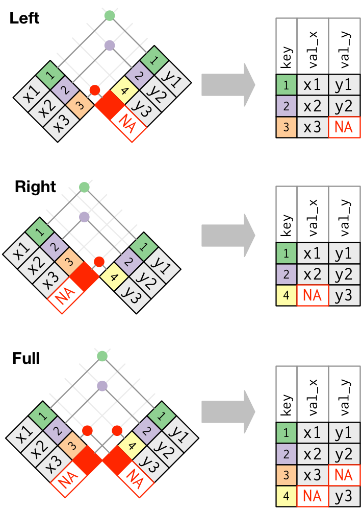
Left joins, right joins, and full joins are also collectively referred to as outer joins because they retain the observations from at least one of the joined tables. This excellent set of diagrams from R for Data Science (R4DS) can help you build an intuitive sense of how these outer joins work:

source: https://r4ds.had.co.nz/relational-data.html

6 inner_join()

Often you may only want to work with rows which have matching entries in both data sources. Since only some rows are retained, we’re no longer dealing with an outer join. In this case you could use inner_join(), which returns all rows in both x and y but only rows with that appear in the key columns of both data frames.

life_df %>% 
  inner_join(gdp_df)

## # A tibble: 8 x 4
##   continent  year mean_life_expectancy total_gdpPercap
##   <fct>     <int>                <dbl>           <dbl>
## 1 Africa     1997                 53.6         123695.
## 2 Africa     2007                 54.8         160630.
## 3 Americas   1997                 71.2         222233.
## 4 Americas   2007                 73.6         275076.
## 5 Europe     1997                 75.5         572303.
## 6 Europe     2007                 77.6         751634.
## 7 Oceania    1997                 78.2          48048.
## 8 Oceania    2007                 80.7          59620.

This time we only get data for 1997 and 2007 even though life_df has values for 2002 because gdp_df did not contain any data for 2002. We also don’t get any data for Asia, which was present in gdp_df, because there was no data for Asia in life_df.

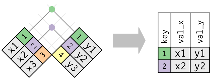
This diagram from R4DS shows you another example of how an inner join works:

source: https://r4ds.had.co.nz/relational-data.html

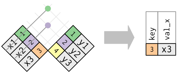
7 semi_join()

So far we’ve been filtering rows based on matches in the key columns but extacting all columns from both data frames. The other two main dplyr join functions are available for situations where you only want to keep the columns of one data frame (x).

semi_join(x, y) filters the rows of x to retain only those that also appear in y

life_df %>% 
  semi_join(pop_df)

## # A tibble: 9 x 3
##   continent  year mean_life_expectancy
##   <fct>     <int>                <dbl>
## 1 Africa     1997                 53.6
## 2 Africa     2002                 53.3
## 3 Africa     2007                 54.8
## 4 Americas   1997                 71.2
## 5 Americas   2002                 72.4
## 6 Americas   2007                 73.6
## 7 Oceania    1997                 78.2
## 8 Oceania    2002                 79.7
## 9 Oceania    2007                 80.7

This time we only get the columns from life_df and we’ve dropped rows for Europe because Europe only appears under the continent key column for life_df and not pop_df.

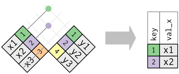
Here is the R4DS semi-join diagram showing that only columns and rows from table 1 are retained as a second example:

source: https://r4ds.had.co.nz/relational-data.html

8 anti_join()

In contrast to semi joins, anti joins return the rows x that do not appear in y.

life_df %>% 
  anti_join(pop_df)

## # A tibble: 3 x 3
##   continent  year mean_life_expectancy
##   <fct>     <int>                <dbl>
## 1 Europe     1997                 75.5
## 2 Europe     2002                 76.7
## 3 Europe     2007                 77.6

As you can see, anti joins can be very useful if you want to know which rows are excluded due to mismatches in the key columns. Checking for consistencies and inconsistencies between data sources is an important part of the data cleaning process and can often help to uncover data entry or coding errors that should be fixed prior to conducting any analyses.

R4DS diagram showing how the anti-join works:

source: https://r4ds.had.co.nz/relational-data.html

9 building data frames using bind_rows() or bind_cols()

If you have two data frames with the same columns, you can combine their rows using dplyr::bind_rows() or rbind(). rbind() is best suited for rowwise combinations of vectors or matrices, while bind_rows() is better for combining data frames. In my experience, the most common reason to use either would be to add data for new cases to a data frame, so I will only demonstrate bind_rows() here. For example, say we decided to add the gapminder life expectancy data for Asia to life_df:

#first get the data for asia from the original gapminder dataset
asia_life_exp <- gapminder %>%
  filter(continent == "Asia",
         between(year, 1997, 2007)) %>% #between is a shortcut for (column >= value & column <= value) 
  group_by(continent, year) %>% 
  summarise(mean_life_expectancy = mean(lifeExp, na.rm = T))

#then add it to the top of life_df
bind_rows(asia_life_exp, life_df) 

## # A tibble: 15 x 3
## # Groups:   continent [5]
##    continent  year mean_life_expectancy
##    <fct>     <int>                <dbl>
##  1 Asia       1997                 68.0
##  2 Asia       2002                 69.2
##  3 Asia       2007                 70.7
##  4 Africa     1997                 53.6
##  5 Africa     2002                 53.3
##  6 Africa     2007                 54.8
##  7 Americas   1997                 71.2
##  8 Americas   2002                 72.4
##  9 Americas   2007                 73.6
## 10 Europe     1997                 75.5
## 11 Europe     2002                 76.7
## 12 Europe     2007                 77.6
## 13 Oceania    1997                 78.2
## 14 Oceania    2002                 79.7
## 15 Oceania    2007                 80.7

If we instead had two data frames with the same cases/rows but different columns (and no common key columns to enable the use of joins), we could combine them using dplyr::bind_cols() or cbind(). Again, bind_cols() is preferred over cbind() for combining data frames by column. However, if you’re only adding a few columns, dplyr::mutate() or a "df$newcol <- newcol" statement per column to add would also work.

For example, if we were provided with each column of the gapminder dataframe as separate vectors (each with values in identical order), without any common key columns among any of the fragments, we could reconstruct the orginal gapminder data frame using bind_cols(), e.g.:

ctry <- gapminder$country

ctin <- gapminder$continent

yr <-  gapminder$year

le <- gapminder$lifeExp

pop <- gapminder$pop

gdp <- gapminder$gdpPercap

bound_gap <- bind_cols("country" = ctry, #add names using "name" = vector syntax
                       "continent" = ctin, 
                       "year" = yr, "lifeExp" = le, 
                       "pop" = pop, 
                       "gdpPercap" = gdp)

identical(gapminder, bound_gap)

## [1] TRUE

#the main difference between cbind() and bind_rows() is that bind_rows returns a
#tibble

When considering the use of rbind()/bind_rows() or cbind()/bind_cols() you must keep in mind that because no key columns are checked for matching values you need to be sure that the columns (when binding rows) or rows (when binding columns) are arranged in exactly the same order for each portion of the dataframe before binding the pieces together. This approach can be very error prone, particularly in cases where data cleaning or analysis is being done collaboratively.

For this reason I strongly recommend that you make use of key columns and combine data using joins whenever possible.

updated_life_df <- life_df %>% 
  tibble::add_row(continent = "Africa", year = 2012, mean_life_expectancy = 56) %>%  #specify values to be added using column = value syntax
  arrange(continent, year)

updated_life_df #now the value we added appears in the printout of the data frame

## # A tibble: 13 x 3
##    continent  year mean_life_expectancy
##    <chr>     <dbl>                <dbl>
##  1 Africa     1997                 53.6
##  2 Africa     2002                 53.3
##  3 Africa     2007                 54.8
##  4 Africa     2012                 56  
##  5 Americas   1997                 71.2
##  6 Americas   2002                 72.4
##  7 Americas   2007                 73.6
##  8 Europe     1997                 75.5
##  9 Europe     2002                 76.7
## 10 Europe     2007                 77.6
## 11 Oceania    1997                 78.2
## 12 Oceania    2002                 79.7
## 13 Oceania    2007                 80.7

10 joining 3 or more data frames

Joining 3 or more data frames is also pretty easy using dplyr, just pipe the output of a join into another join. This is incredibly simple if they all have key columns with the same names. For example, if I wanted to combine life_df, pop_df and gdp_df and keep rows present in any of them, all I have to do is:

combined_data <- life_df %>% 
  full_join(pop_df) %>% #life_df is inserted as the 1st argument i.e. data frame "x" of the full_join
  full_join(gdp_df) #the output of the previous join is passed to the first argument of the second full_join

combined_data #now it's all together, using what could be condensed into a single line of code

## # A tibble: 15 x 5
##    continent  year mean_life_expectancy total_population total_gdpPercap
##    <fct>     <int>                <dbl>            <dbl>           <dbl>
##  1 Africa     1997                 53.6        743832984         123695.
##  2 Africa     2002                 53.3        833723916             NA 
##  3 Africa     2007                 54.8        929539692         160630.
##  4 Americas   1997                 71.2        796900410         222233.
##  5 Americas   2002                 72.4        849772762             NA 
##  6 Americas   2007                 73.6        898871184         275076.
##  7 Europe     1997                 75.5               NA         572303.
##  8 Europe     2002                 76.7               NA             NA 
##  9 Europe     2007                 77.6               NA         751634.
## 10 Oceania    1997                 78.2         22241430          48048.
## 11 Oceania    2002                 79.7         23454829             NA 
## 12 Oceania    2007                 80.7         24549947          59620.
## 13 Asia       1997                 NA         3383285500         324525.
## 14 Asia       2002                 NA         3601802203             NA 
## 15 Asia       2007                 NA         3811953827         411610.

# Alternatively, I could use full_join(life_df, pop_df) %>% full_join(gdp_df)

# or full_join(full_join(life_df, pop_df), gdp_df)

This is another example of how nested function calls can be easier to read when written in series with the pipe operator (%>%), which I covered in more detail here.

11 merge()

In the very unlikely event that you find yourself having to combine relational data but are working on a computer that only has base R and no admin priviledges to enable you to install dplyr, have no fear! You can use the merge() function from base R to perform left joins, right joins, inner joins, and full joins.

In addition to the x and y arguments that need to be used to specify the data frames to be joined and the by argument that indicates which key columns to use, the type of join is determined via the all.x and all.y arguments

# inner join/merge

ij_merge <- merge(life_df, pop_df,
            all.x = F, all.y = F) #the default merge/join is an inner join, in which all.x and all.y are both FALSE

ij_dplyr <- inner_join(life_df, pop_df) %>% 
  as.data.frame() #removes the tibble class which the merge result doesn't have

all.equal(ij_merge, ij_dplyr)

## [1] TRUE

#full join/merge
fj_merge <- merge(life_df, pop_df,
            all.x = T, all.y = T) #set (all.x = T and all.y = T) or (all = T), to perform a full join

fj_dplyr <- full_join(life_df, pop_df) %>% 
  as.data.frame() %>%
  arrange(continent)

all.equal(fj_merge, fj_dplyr)

## [1] TRUE

#for a left join, all.x should be set to TRUE and all.y to FALSE
lj_merge <- merge(life_df, pop_df,
            all.x = T, all.y = F) 

lj_dplyr <- left_join(life_df, pop_df) %>% as.data.frame()

all.equal(lj_merge, lj_dplyr)

## [1] TRUE

#for a right join, all.x should be set to FALSE and all.y to TRUE
rj_merge <- merge(life_df, pop_df,
            all.x = F, all.y = T) 

rj_dplyr <- right_join(life_df, pop_df) %>% as.data.frame()

all.equal(rj_merge, rj_dplyr)

## [1] "Component \"continent\": 6 string mismatches"                                        
## [2] "Component \"mean_life_expectancy\": 'is.NA' value mismatch: 3 in current 3 in target"
## [3] "Component \"total_population\": Mean relative difference: 1.974144"

Why bother with dplyr joins if merge() can do so much? Simply because the dplyr code is easier to read and the dplyr functions are faster. Unfortunately, merge also can’t handle semi joins or anti joins, so you’d have to do a bit more work to achieve the same results without dplyr.

If you’ve followed along, congratulations! You now know how the basics of combining data frames in with dplyr joins and base R. Just practice these operations a few times on your own and joins will seem trivial!

12 Navigation

Click here to go back to the previous post on reshaping data with tidyr or here to go to the next post on string manipulation with stringr.

13 Notes

• You can learn more about joins, working with relational data, and the set operation functions in R here.

• You can learn more about SQL here.

• The author of dplyr, Hadley Wickham, also wrote the dbplyr package, which translates dplyr to SQL for you so you can actually query databases directly using dplyr code or even view the SQL code translations. You can learn more about dbplyr here. The code translation is really helpful if you’re trying to learn SQL.

Thank you for visiting my blog. I welcome any suggestions for future posts, comments or other feedback you might have. Feedback from beginners and science students/trainees (or with them in mind) is especially helpful in the interest of making this guide even better for them.

This blog is something I do as a volunteer in my free time. If you’ve found it helpful and want to give back, coffee donations would be appreciated.